From: John Conover <john@email.johncon.com>
Subject: Data Set Size Requirements for Equity Price Analysis
Date: 9 Jan 2001 02:14:50 -0000
Entropic analysis can provide data set size requirements for equity price analysis-in other words, how long a stock's performance must be measured to produce a reliable estimate of the stock's investment potential. Underestimating data set size requirements is the most common investment mistake-made even by professional traders. In point of fact, determining data set size requirements is not trivial, and traditional rule-of-thumb methods can often produce misleading results.
To delve into the issue, I will describe the methods used in the tsinvest program. The tsinvest program is not a replacement for investment due diligence-it is an automated "graph watcher" that extends the depth a breadth of the investing horizon; it is capable of determining the price performance characteristics of hundreds of thousands of stocks a day, and automatically compensates those characteristics for inadequate data set size requirements.
Using the Efficient Market Hypothesis, (EMH, as suggested by Louis Bachelier in 1900, Theorie de la Speculation,) model as a first order approximation to equity prices, the marginal return of a stock on the n'th day is:
    V(n)  - V(n - 1)
    ---------------
        V(n - 1)
where V(n) is the stock's price on the n'th day, and V(n - 1) is the price on the preceding day. The average marginal return, avg, over an interval of N many days is the sum of the daily marginal returns, divided by N.
The standard deviation of the marginal returns, rms, over an interval of N many days is the square root of 1 / N times the sum of each daily marginal return squared.
Using information-theoretic methodologies, (following J. L. Kelly, Jr., A New Interpretation of Information Rate) it can be shown that the Shannon probability, (i.e., the likelihood of an up movement in a stock's price, named after Claude Shannon's pioneering work in the mid 1940's, The Mathematical Theory of Communication,) P, on any day is:
        (avg / rms) + 1
    P = ---------------
              2
and the average daily gain in a stock's value, G, is:
G = ((1 + rms)^P) * ((1 - rms)^(1 - P))
A complete derivation of these equations can be found in the tsinvest on line manual page, which also contains a suitable bibliography.
As a side bar, note that if avg = rms, then:
P = 1
and:
G = (1 + avg)
meaning that the likelihood of an up movement is 100%, (a certainty,) and the gain per day would be 1 + avg; or for N many days, (1 + avg)^N, which is the formula for compound interest.
So in some sense, the EMH assumes a compound interest model of equity prices-only the interest rate, (e.g., the daily marginal returns,) is not fixed, (and can even be negative,) and can not be known in the future. The only requirement imposed by the EMH is that the daily marginal returns have a normal/Gaussian distribution, (with a mean of avg, and a standard deviation of rms.)
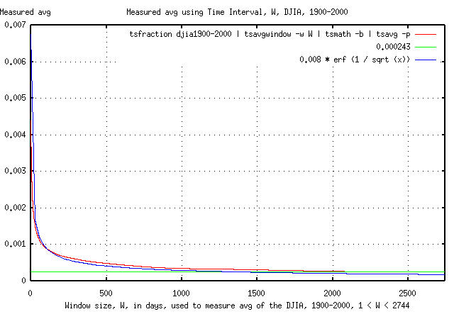
As an example, using the daily returns of the Dow Jones Industrial Average, (DJIA,) for January 2, 1900 through December 29, 2000, and using the tsfraction, tsavg, and tsrms programs (from the tsinvest Utilities page,) to calculate the avg and rms of the DJIA:
tsfraction djia1900-2000 | tsavg -p
0.000243
and:
tsfraction djia1900-2000 | tsrms -p
0.010948
meaning that the average daily marginal return for the 101 years was 0.000243, and that for one standard deviation, (i.e., 68.27% of the time,) the daily fluctuations in the value of the DJIA were less than +/- 0.010948, or about 1%.
The Shannon probability, P, of the DJIA would be:
P = ((0.000243 / 0.010948) + 1) / 2 = 0.51109791743
or the index increased in value about 51 out of a 100 days, on average, over the 101 years.
The daily gain, G, in value of the DJIA would be:
    G = ((1 + 0.010948)^0.51109791743)
        * ((1 - 0.010948)^(1 - 0.51109791743))

      = 1.00018309353
or, on average, the DJIA increased in value about 0.02% per trading day, or 4.7% per year, over the 101 years.
(As a cross check, there were 27,659 trading days in the 101 year period, and 1.00018309353^27659 = 158.177906992-or the DJIA increased about 158X in the 101 year period; on January 2, 1900, the DJIA was 68.13, and 68.13 * 158.177906992 = 10,776.6608034; the value on December 29, 2000 was 10787.99-which is reasonably close, within about a tenth of a percent.)
Note that only the average, avg, and root mean square, rms, of the daily marginal returns are used in the calculation of the value of the index, G.
But was the accuracy of these numbers adequate?
Fortunately, Jakob Bernoulli, (Ars Conjectandi, 1713,) and Abraham de Moivre a few years later, (The Doctrine of Chances,) answered the question when they formalized the Law of Large Numbers, (which was later to become the theory of the Gaussian Bell Curve, even though Gauss didn't have anything to do with it.)
The way Bernoulli and de Moivre approached the problem was by analyzing the convergence of repeated trial data. For example, if one wanted to verify that a tossed coin was fair, (i.e., 50/50 chance of coming up heads or tails,) one could toss a coin many times, counting the number of times it comes up heads, and divide it by the total trials. But exactly how would the data converge to 0.5?
As it turns out, after a lot of formalism, the convergence is described by the error function, erf, and is erf (1 / sqrt (N)).
This remarkable conclusion can be reasoned out, intuitively. When we add random things, like trials, together, we add them by the square root of the sums of their standard deviations, squared. So, we would expect repeated trial data to increase proportional to the square root of the number of trials, sqrt (N). However, when we average this data, we divide it by the number of trials, N, so that the convergence would be proportional sqrt (N) / N, which is 1 / sqrt (N). And for N >> 1, erf (1 / sqrt (N)) is about 1 / sqrt (N).
So, as a simple example, we would expect a person that plays a game of tossing a fair coin, and taking one step left if it comes up heads, or one step right if it comes up tails, to be the sqrt (N) steps away from the origin after N many tosses of the coin. (In point of fact, if the game was iterated, we would expect that in one standard deviation of the games, or 68.27%, the person was less than sqrt (N) steps away from the origin.) If, indeed, the coin was fair, erf (1 / sqrt (N)) would converge to zero.
Note the similarity to the process prescribed by the EMH, where to get today's value of an index, we select a random number from a Gaussian distribution with a standard deviation of rms, then add to that selection an offset of avg, and then add that to yesterday's value.
Note that fractal concepts are not new-such things as self-similarity, were described by Bernoulli and de Moivre almost three centuries ago. Self-similarity means that the same statistics hold true, even if N is multiplied by a constant, (i.e., if we measure things at N, or 10 * N, or 100 * N, or any multiplier, the square root characteristics will still hold; a very counter intuitive conclusion.)
As an example of self similarity, the answer to the question of how long equity market "bubbles" last is that half last less than t time units, where 1 / sqrt (t) = 0.5, and half more; or where t is about 4 years when years are used as the time scale. It is true for decades, months, weeks, days, hours, and minutes, too. So, in some sense, equity prices are fractal, and made up of "micro-bubbles," which assemble their self into "milli-bubbles," which assemble their self into "bubbles", and so on, with all the "bubbles" having 1 / sqrt (t) duration distributions, and sqrt (t) magnitude distributions.
Note that this implies that there is a science to equity market "bubbles", and that we have answered the question concerning the accuracy of the numbers derived in the analysis of the DJIA, above.
To illustrate the point, Figure I is a graph of the convergence of the average of the marginal returns avg, of the DJIA, as it converges to its average value of 0.000243. A graph of the theoretical convergence, erf (1 / sqrt (x)), is superimposed for comparison.
Note that the analysis requires several years of daily data to determine the value of avg with reliable accuracy. Making an investment decision on a smaller data set size could lead to very optimistic estimates.
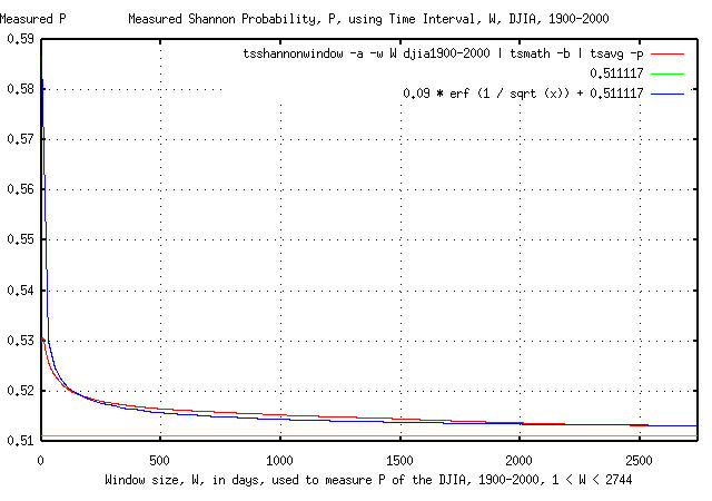
Since, for typical stocks on the US exchanges, the convergence of the Shannon probability, P, is dominated by the convergence of avg, the convergences of P and avg would be expected to be similar. Figure II is a graph of the convergence of the Shannon probability, P, calculated using the daily marginal returns of the DJIA, as it converges to its average value of 0.51109791743. A graph of the theoretical convergence, erf (1 / sqrt (x)), is, again, superimposed for comparison.
The convergence of the root mean square of the daily marginal returns, rms, of the DJIA is shown in Figure III.
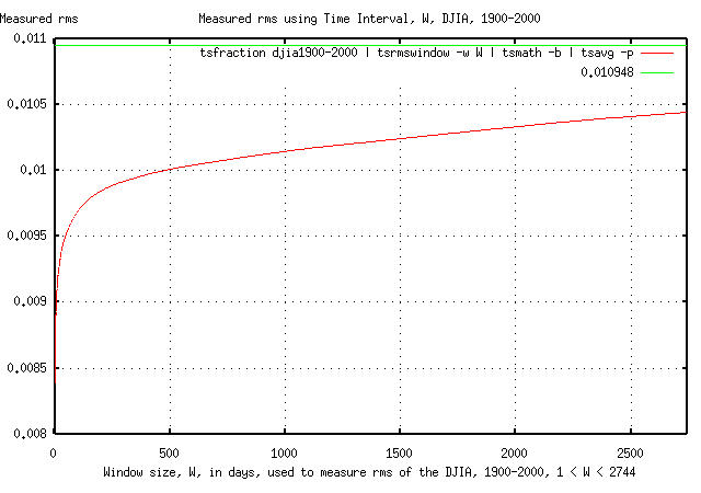
Note that the convergence of the Shannon probability, P, is dominated by the convergence of the average of the daily marginal returns, avg; the root mean square of the daily marginal returns, rms, approaching a modest 10% error in 211 days vs. 1,894 days required for the same error in the avg.
Note that the root mean square of the daily marginal returns, rms, has a slightly different meaning in this presentation than described in classical Black-Scholes methodologies. In Black-Scholes, rms is a metric of risk, and is calculated by subtracting the mean, avg, from each element in the calculation of the rms time series. In the special case of compound interest, the Black-Scholes methodology would have rms = zero, (i.e., no risk.) However, it is advantageous to work with probabilities-where, in the corresponding case of compound interest, the likelihood of an up movement, P, is unity.
Although the methods are similar, it is possible to accommodate inadequate data set size risks in an investment strategy by combining the probabilities.
For example, would investing on the DJIA index, (i.e., a derivative,) with only 100 days of data be a wise "wager"?
The combined probabilities, P' can be approximated by:
    P' = P * (1 - 1 / sqrt (t)) = 0.52 * (1 - 1 / sqrt (100)
       = 0.468
where P = 0.52 is a representative Shannon probability, (i.e., a "typical" value, obtained by measuring P on all 100 day intervals in the 20'th century,) from Figure II, at W = 100 days. So, the answer would be no, (at least from the EMH point of view,) since at least a 50/50 chance of winning is required for any reasonable "wager," (another of mathematics most profound insights.)
The minimum data set size for the DJIA can be calculated:
0.5 = 0.51109791743 * (1 - 1 / sqrt (t))
or:
t = 2,120.9246719
trading days, which is over eight calendar years!
Compare this against the overly optimistic calculated gain in index value, G, when based on the 100 day values, P = 0.52, and rms = 0.0097, from Figures II and III:
    G = ((1 + 0.0097)^0.52) * ((1 - 0.0097)^(1 - 0.52))
      = 1.00034102309
which is an average of 9% gain per year-a very optimistic factor of 2 over the 4.7% that the DJIA actually did!
Bear in mind that this does not mean that a long term investor basing decisions on smaller data set sizes will lose money. It does mean, however, that an investor that does so will not make as much money consistently.
Note that such probabilistic methodologies are similar to standard statistical estimation techniques, and in some sense, perform a "low pass filter," function that reduces the effect of market "bubbles" to an acceptable value when using metric techniques that rely on the EMH as a model for stock price analysis.
As a cross check, for such a scheme to work, it would seem intuitively reasonable that market "bubbles" in the DJIA have to exhibit the same erf (1 / sqrt (t)) characteristics that were probabilistically filtered. Figure IV is a graph of the combined "bull" and "bear" market "bubbles" for the DJIA daily closes, January 2, 1900 through December 29, 2000.
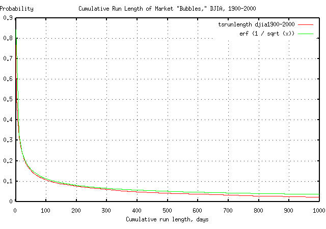
The graph in Figure IV was made with the tsrunlength program, (from the from the tsinvest Utilities page.) As an example usage of Figure IV, suppose that today, the DJIA increased in value. What are the chances that the increase will turn into a "bubble" lasting at least a hundred trading days? About 10%. Using 1 / sqrt (t) as an approximation to erf (1 / sqrt (t)), for t >> 1, 1 / sqrt (100) = 0.1, or about 10%.
Which is a handy way of looking at equity market "bubbles," and might have precluded many investors from over extendeding their "dot-com" portfolio asset allocations.
--

John Conover, john@email.johncon.com, http://www.johncon.com/