Verification of Analytical Methodology for Evaluating GDP Per Capita:
To demonstrate the validity of the analytical methodology
used in the GDP per capita analysis, tsinvestsim(1)
simulations were used to evaluate the convergence of the log-normal
distribution of GDP per capita with population sizes over
five orders of magnitude, (N =
10 to N =
100,000,) and each worker in the workforce
having P = 0.51, f
= rms = 0.02 * 0.5 * 0.41, representing a
maximally optimal efficiency, (P =
0.51, f = rms =
0.02,) with an inefficiency of
0.41 representing the fraction
of the population in the workforce, and each worker in the
workforce operating with an inefficiency of
0.5. These variable values are
representative for the daily values, per worker, of
many industrialized nations.
The output of the tsinvestsim(1)
program was summed into an aggregate GDP using the tsinvestsim-lognormal(1)
program, (source
archive,) to obtain the
mean,
median, and
mode of the simulated GDP, as a
time
series, with a log-normal
distribution, i.e., the GDP per capita distribution.
Since economic data for productivity is available only on a
per capita basis, it is not feasible to determine the
inefficiencies, (they are lumped together.) The
methodology used allows simulations with different variable
values for P, f =
rms, and
avg. For the current
simulations, it is assumed that each worker in the workforce
can operate maximally optimal, P =
0.51, and f = rms =
0.02, (f^2 = rms^2 =
avg, which is maximally optimal, subject to
the Kelly
Criteria,) and f = rms is
decreased to represent the inefficiencies. Note that this
decreases avg by the same
inefficiency factor:
P = ((avg / (k * rms)) + 1) / 2
avg = (k * rms) * ((2 * P) - 1)
Where P is invariant with
k,
(avg is computed by the tsinvestsim(1)
program in this manner) Note, further, that:
rms = sqrt (srms^2 + avg^2)
k * rms = k * sqrt (srms^2 + avg^2)
k * rms = sqrt ((k^2 * srms^2) + (k^2 * avg^2))
k * rms = sqrt ((k * srms)^2 + (k * avg)^2)
indicating that rms can be
multiplied by a constant, k,
without first calculating srms
and avg, then multiplying each
by k, squaring each product, and
finally taking the root-mean-square of the sum of the
squares.
The rationale for selecting variable values in this manner
is that P is a metric on a
worker's ability to synthesize innovation based on new
information, (original, secret, or public,) and
f = rms is a metric on the
wager made on the innovation, with
avg being the return, (positive
or negative,) generated by the innovation, i.e., metrics on
how smart the worker is, and how good a gambler.
If the national GDP per capita, (an aggregate expenditure
approach,) and distribution of income, (an aggregate income
approach,) are analyzed together, the variable values for a
typical worker in the economy can be determined.
In the following simulations, all workers have the same
daily variable values P = 0.51,
and f = rms = 0.02 * 0.5 * 0.41,
(for 51 times out of a hundred innovation success rate, 50%
efficiency at wagering, and 41% of the population in the
workforce,) with each worker starting at I =
$10, (all equal, representing the rural/shared
agricultural economy of the US in 1610,) and the simulations
are all allowed to run for 100,000 days, (about 4 centuries at
250 work days a year,) developing into a log-normal
distribution standard of living, (i.e., GDP growth per
capita,) by 1790, and continuing through 2010. The simulation
outputs are then sampled every 250 days, for annual data, and
all values filtered, prior to 1790, resulting in 1790 through
2010 annual data. The simulation was repeated for workforce
sizes of N = 10, N
= 100, N =
1,000, N =
10,000, and N =
100,000, to verify convergence to the mean of
the simulations.
It should be pointed out, as a concluding remark, that the
objective of the simulations are validity of methodology which
requires only a reasonable approximation to the actual US GDP
per capita-and two digit precision variables is adequate.
Analysis of Simulations:
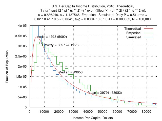
Figure I
Figure I is a plot of the US nominal GDP per capita income
distribution, 2010: theoretical distribution, empirical
distribution, and, simulated distribution (N =
100,000.)
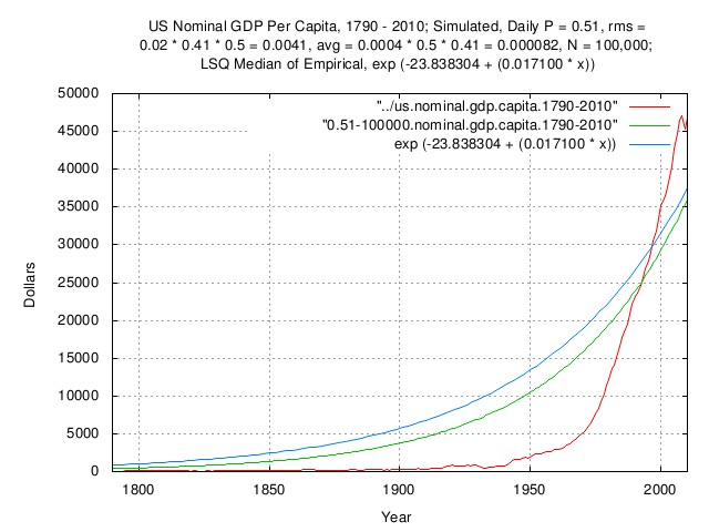
Figure 2
Figure 2 is a plot of the US nominal GDP per capita,
1790-2010: empirical values, simulated values (N
= 100,000,) and Least Squares fit of the
empirical values.
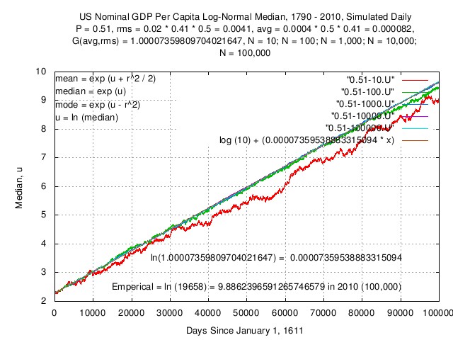
Figure III
Figure III is a plot of the simulated US GDP per capita
log-normal
distribution median, over time, with five orders of magnitude of
population sizes, N, and a plot
of the theoretical values for N =
100,000. Note the convergence to the
theoretical values with increasing
N. Further, note that the values
converged to are independent of
N:
P = 0.51
rms = 0.02 * 0.5 * 0.41
avg = (rms) * ((2 * P) - 1)
= 0.000082
G(avg,rms) = 1.00007359809704021647
Or, the value, V, at a time
x many days, starting with an
initial value of I = 10:
V(x) = I * G(avg,rms)^x
Or:
ln (V(x)) = ln (10) + (x * ln (G(avg,rms)))
= 2.30258509299404568402 + (0.00007359538883315094 * x)
It is important to note that this represents the aggregate
growth in the median of the workforce divided by the size of
the population, (i.e., the median per capita value,) over
time, with the workforce operating at 50% efficiency,
(relative to rms,) and has a
direct mathematical relationship to the typical
worker variable values, rms and
P, on a daily basis. This
function is exponentiated to obtain the median of the log-normal
distribution, over time.
Figure IV
Figure IV is a plot of the simulated US nominal GDP per
capita log-normal
distribution deviation, over time, with five orders of
magnitude of population sizes,
N, and a plot of the theoretical
values for N = 100,000. Note the
convergence to the theoretical values with increasing
N. Further, note that the values
converged to are independent of
N:
P = 0.51
rms = 0.02 * 0.5 * 0.41
avg = (rms) * ((2 * P) - 1)
= 0.000082
srms = sqrt (rms^2 - avg^2)
= 0.0040991799179835959
Or, the value, S, at a time
x many days:
S(x) = srms * sqrt (x)
= 0.0040991799179835959 * sqrt (x)
It is important to note that this represents the standard
deviation of the Gaussian/Normal distribution of the standard
of living of the workforce (i.e., the distribution of the per
capita values,) over time, with the workforce operating at 50%
efficiency, (relative to rms,)
and has a direct mathematical relationship to the
typical worker variable values,
rms and
P, on a daily basis. The square
of this function, divided by two, is exponentiated to obtain
the deviation from the median of the log-normal
distribution, over time.
Further, it is important to note that the
srms of the workers, (or their
typical value of the aggregate,) is related to the
median and mean of the log-normal
distribution at any time.
Analytical Methodology:
Let t be the time interval
the log-normal
distribution has evolved in the data file,
data.file, of the GDP
per capita. Then, in the t'th,
(last,) interval:
u = Mu
r = Rho
median = e^u
mean = e^(u + (r^2 / 2))
mode = e^(u - r^2)
If the data.file
represents GDP per capita data, (i.e., annual GDP divided by
annual population count,) then the file represents
mean GDP per capita
data. One of the issues is to convert the data to
median data.
It is convenient to analyze the evolution of log-normal
distribution, meaning by time,
t:
median(t) = e^u(t)
mean(t) = e^(u(t) + (r(t)^2 / 2))
mode(t) = e^(u(t) - r(t)^2)
where for economic data, (like the US GDP per capita,) the
mean(t) historical time
series and the median(t),
mean(t), and
mode(t) are available only at
one point in time, (usually the last interval.)
mean(t) = e^(u(t) + (r(t)^2 / 2))
mode(t) = e^(u(t) - r(t)^2)
mean(t) = e^(u(t)) * e^(r(t)^2 / 2)
mode(t) = e^(u(t)) / e^(r(t)^2)
mean(t) / mode(t) = (e^(u(t)) * e^(r(t)^2 / 2)) / (e^(u(t)) / e^(r(t)^2))
mean(t) / mode(t) = (e^(r(t)^2 / 2)) / (1 / e^(r(t)^2))
mean(t) / mode(t) = (e^(r(t)^2 / 2)) * e^(r(t)^2)
mean(t) / mode(t) = e^((r(t)^2 / 2) + r(t)^2)
mean(t) / mode(t) = e^(r(t)^2 * (1 + (1 / 2)))
mean(t) / mode(t) = e^((3 / 2) * r(t)^2)
ln (mean(t) / mode(t)) = (3 / 2) * r(t)^2
r(t)^2 = (2 / 3) * ln (mean(t) / mode(t))
r(t) = sqrt ((2 / 3) * ln (mean(t) / mode(t)))
r(t) = srms * sqrt (t)
r(t)^2 = srms^2 * t
mean(t) = e^(u(t) + (r(t)^2 / 2))
u(t) = a + (b * t)
mean(t) = e^(a + (b * t) + (srms^2 * t / 2))
mean(t) = e^(a + (b * t) + ((srms^2 / 2) * t))
mean(t) = e^(a + ((b + (srms^2 / 2)) * t))
median(t) = e^u(t) = e^(a + (b * t))
with a and
b determined by LSQ of
mean(t).
Validation:
Unfortunately, the tsinvestsim-lognormal(1)
program does not provide the
mode(t) but as an alternative
derivation using the median(t)
and mean(t) for analysis of the
simulation:
mean(t) = e^(u(t) + (r(t)^2 / 2))
mean(t) = e^u(t) * e^(r(t)^2 / 2)
median(t) = e^u(t)
mean(t) = e^u(t) * e^(r(t)^2 / 2)
mean(t) / median(t) = e^u(t) * e^(r(t)^2 / 2) / e^u(t)
mean(t) / median(t) = e^(r(t)^2 / 2)
r(t)^2 / 2 = ln (mean(t) / median(t))
r(t)^2 = 2 * ln (mean(t) / median(t))
r(t) = sqrt (2 * ln (mean(t) / median(t)))
r(t) = srms * sqrt (t)
srms = r(t) / sqrt (t)
mean(t) = e^(a + ((b + (srms^2 / 2)) * t))
ln (mean(t)) = a + ((b + (srms^2 / 2)) * t)
The actual values used in the simulation:
P = 0.51, f = 0.02 * 0.50 * 0.41 = 0.0041
f = rms = 0.02 * 0.50 * 0.41 = 0.0041
0.51 = ((avg / 0.0041) + 1) / 2
avg = 0.0041 * ((2 * 0.51) - 1)
= 0.000082
srms = sqrt (rms^2 - avg^2)
= sqrt (0.0041^2 - 0.000082^2)
= 0.0040991799179835959
G(avg,rms) = G(0.0041 * ((2 * 0.51) - 1),0.02 * 0.50 * 0.41)
= 1.00007359809704021647
G(t) = 10 * (1.00007359809704021647^t)
ln (G(t)) = ln (10) + (t * ln (1.00007359809704021647))
= 2.30258509299404568402 + (0.00007359538883315094 * t)
ln (mean(t)) = a + ((b + (srms^2 / 2)) * t)
a = 2.30258509299404568402
b + (srms^2 / 2) = 0.00007359538883315094
b = 0.00007359538883315094 - (srms^2 / 2)
= 0.00007359538883315094 - (0.0040991799179835959^2 / 2)
= 0.00006519375083315094
ln(mean(t)) = 2.30258509299404568402 + (0.00007359538883315094 * t)
And, analyzing the data from the simulations, (the order of
the fields from tsinvestsim-lognormal(1)
program): "time,
minimum,
median,
mean,
maximum",):
cut -f4 0.51-10 | tslsq -e -p
e^(2.243692 + 0.000091t)
cut -f4 0.51-10 | tsfraction | tsavg -p
0.000089
cut -f4 0.51-10 | tsfraction | tsrms -p
0.002662
G(0.000089,0.002662) = 1.00008546072723226738
ln (G(0.000089,0.002662)) = 0.00008545707567235967
egrep '^99999' 0.51-10
99999 1906.627099 8477.783394 52569.322616 387424.213469
r(100000) = sqrt (2 * ln (52569.322616 / 8477.783394))
= 1.91033175441258050009
srms = 1.91033175441258050009 / sqrt (100000)
= 0.00604099943048917012
r(t) = srms * sqrt (t)
r(t) = 0.00604099943048917012 * sqrt (t)
r(t)^2 / 2 = 0.00001824683705958524 * t
ln (mean(t)) = a + ((b + (srms^2 / 2)) * t)
a = 2.243692
b = 0.000091 - (0.00604099943048917012^2 / 2)
= 0.00007275316294041476
u(t) = 2.243692 + (0.00007275316294041476 * t)
cut -f4 0.51-100 | tslsq -e -p
e^(2.230331 + 0.000083t)
cut -f4 0.51-100 | tsfraction | tsavg -p
0.000084
cut -f4 0.51-100 | tsfraction | tsrms -p
0.000736
G(0.000084,0.000736) = 1.00008373267247867903
ln (G(0.000084,0.000736)) = 0.00008372916709413426
egrep '^99999' 0.51-100
99999 290.545725 12589.060312 43569.000789 1248187.418192
r(100000) = sqrt (2 * ln (43569.000789 / 12589.060312))
= 1.57576501978003208644
srms = 1.57576501978003208644 / sqrt (100000)
= 0.00498300651972517984
r(t) = srms * sqrt (t)
r(t) = 0.00498300651972517984 * sqrt (t)
r(t)^2 / 2 = 0.00001241517698781182 * t
ln (mean(t)) = a + ((b + (srms^2 / 2)) * t)
a = 2.230331
b = 0.000083 - (0.00498300651972517984^2 / 2)
= 0.00007058482301218818
u(t) = 2.230331 + (0.00007058482301218818 * t)
cut -f4 0.51-1000 | tslsq -e -p
e^(2.289082 + 0.000082t)
cut -f4 0.51-1000 | tsfraction | tsavg -p
0.000083
cut -f4 0.51-1000 | tsfraction | tsrms -p
0.000220
G(0.000083,0.000220) = 1.00008297924392550143
ln (G(0.000083,0.000220)) = 0.00008297580133848107
egrep '^99999' 0.51-1000
99999 101.798190 15302.138722 38246.692966 987378.496244
r(100000) = sqrt (2 * ln (38246.692966 / 15302.138722))
= 1.35356159353659762681
srms = 1.35356159353659762681 / sqrt (100000)
= 0.00428033758890269486
r(t) = srms * sqrt (t)
r(t) = 0.00428033758890269486 * sqrt (t)
r(t)^2 / 2 = 0.00000916064493748667 * t
ln (mean(t)) = a + ((b + (srms^2 / 2)) * t)
a = 2.289082
b = 0.000082 - (0.00428033758890269486^2 / 2)
= 0.00007283935506251333
u(t) = 2.289082 + (0.00007283935506251333 * t)
cut -f4 0.51-10000 | tslsq -e -p
e^(2.299558 + 0.000082t)
cut -f4 0.51-10000 | tsfraction | tsavg -p
0.000082
cut -f4 0.51-10000 | tsfraction | tsrms -p
0.000105
G(0.000082,0.000105) = 1.00008199784944121253
ln (G(0.000082,0.000105)) = 0.00008199448780131961
egrep '^99999' 0.51-10000
99999 173.857625 15894.484298 36704.069587 1771254.349566
r(100000) = sqrt (2 * ln (36704.069587 / 15894.484298))
= 1.29376619780877467417
srms = 1.29376619780877467417 / sqrt (100000)
= 0.00409124794481167259
r(t) = srms * sqrt (t)
r(t) = 0.00409124794481167259 * sqrt (t)
r(t)^2 / 2 = 0.00000836915487296287 * t
ln (mean(t)) = a + ((b + (srms^2 / 2)) * t)
a = 2.299558
b = 0.000082 - (0.00409124794481167259^2 / 2)
= 0.00007363084512703713
u(t) = 2.299558 + (0.00007363084512703713 * t)
cut -f4 0.51-100000 | tslsq -e -p
e^(2.300291 + 0.000082t)
cut -f4 0.51-100000 | tsfraction | tsavg -p
0.000082
cut -f4 0.51-100000 | tsfraction | tsrms -p
0.000085
G(0.000082,0.000085) = 1.00008199974949315241
ln(G(0.000082,0.000085)) = 0.00008199638769747028
egrep '^99999' 0.51-100000
99999 39.190364 15804.790282 36694.603142 11503692.146641
r(100000) = sqrt (2 * ln (36694.603142 / 15804.790282))
= 1.29793421590474711612
srms = 1.29793421590474711612 / sqrt (100000)
= 0.00410442837532374379
r(t) = srms * sqrt (t)
r(t) = 0.00410442837532374379 * sqrt (t)
r(t)^2 / 2 = 0.00000842316614408135 * t
ln (mean(t)) = a + ((b + (srms^2 / 2)) * t)
a = 2.300291
b = 0.000082 - (0.00410442837532374379^2 / 2)
= 0.00007357683385591865
u(t) = 2.300291 + (0.00007357683385591865 * t)
Note that:
tsfraction data.file | tsrms -p
rms
is meaningless, (as far as productivity per capita is
concerned,) since the natural evolution of the log-normal
distribution of the aggregate GDP per capita, will be,
given enough time and population, a near perfect exponential
where avg = rms, and
P = 1. The
rms of the workers, (or per
capita value of the aggregate,) must be determined from the
mean(t),
mode(t), and the
median(t) of the distribution at
some time interval, t, (usually
the last interval.)
Empirical GDP per capita data can present situations where
the long term avg and
rms are not nearly equal, which
is usually due to governance issues that effect all, (or
most,) of the workforce, and rms
is greater than
avg. Subtracting, (via
root-mean-square,) the typical individual
rms from the GDP per capita
rms offers a methodology for
analysis of the governance issues, providing the log-normal
distribution has evolved for a sufficient time, and the
population size is sufficiently large.
Simulation:
As a concluding note, to align the simulations,
(mean-variance simulations of geometric Brownian motion
fractals are notoriously unstable,) with the empirical data, 4
data points had to align with the empirical data: the mean of
the simulated nominal US GDP per capita with the empirical
nominal US GDP per capita at 1790; the simulated nominal US
GDP per capita with the empirical nominal US GDP per capita at
2010; and the median; and mean of the log-normal
distribution of the productivity/income of the simulated
nominal US GDP per capita with the empirical nominal US GDP
per capita at 2010. There are 3 variables, which interact:
I, the starting value for each
worker, (I = $10, in 1610, which
was used as a scaling factor);
avg; and,
rms. Lowering both
avg and
rms will decrease the ratio of
the mean to the median in 2010, and, increasing
avg, relative to
rms, will increase the growth in
the nominal US GDP per capita in the simulation. The number of
workers, N, contributing to the
simulated nominal US GDP per capita was increased, in steps of
orders of magnitude, until the simulations converged to their
mean, indicating sufficient accuracy for comparison with the
empirical data. Note that the log-normal
distribution income empirical data for 2010 is in 2010
nominal dollars, necessitating an analysis of nominal US GDP
per capita, (as opposed to the traditional real GDP per
capita.) The empirical log-normal
distribution income in 1790 is not available or known,
necessitating starting the simulation about two centuries
before any data of interest to the analysis to allow a log-normal
distribution income to evolve by 1790. The tsinvestsim(1)
program from the NtropiX
site, (in the tsinvest
archive,) was used to generate the individual worker and
nominal US GDP per capita time
series for the simulation. The simulation for
N = 100,000 took about 20 hours
on a 2.5GHz machine.
calc(1) Macros:
The following calc(1)
macros were used for calculation of
P(avg,rms) and
G(avg,rms) in ~/.calcrc:
    define P (avg, rms) = ((avg / rms) + 1) / 2;
    define G (avg, rms) = power (1 + rms, ((avg / rms) + 1) / 2) * \
                          power (1 - rms, 1 - ((avg / rms) + 1) / 2);
The following calc(1)
script is for computing avg,
rms, and,
G(avg,rms), given
srms and
G obtained empirically from a time
series.
    #!/usr/local/bin/calc -d -f
    #
    # A license is hereby granted to reproduce this design for personal,
    # non-commercial use.
    #
    # THIS DESIGN IS PROVIDED "AS IS". THE AUTHOR PROVIDES NO WARRANTIES
    # WHATSOEVER, EXPRESSED OR IMPLIED, INCLUDING WARRANTIES OF
    # MERCHANTABILITY, TITLE, OR FITNESS FOR ANY PARTICULAR PURPOSE.  THE
    # AUTHOR DOES NOT WARRANT THAT USE OF THIS DESIGN DOES NOT INFRINGE
    # THE INTELLECTUAL PROPERTY RIGHTS OF ANY THIRD PARTY IN ANY COUNTRY.
    #
    # So there.
    #
    # Copyright (c) 1992-2015, John Conover, All Rights Reserved.
    #
    # Comments and/or problem reports should be addressed to:
    #
    #     john@email.johncon.com
    #
    #     http://www.johncon.com/john/
    #     http://www.johncon.com/ntropix/
    #     http://www.johncon.com/ndustrix/
    #     http://www.johncon.com/nformatix/
    #     http://www.johncon.com/ndex/
    #
    # A calc(1) script for binary search-for-solution of: given, srms and
    # g; find avg, rms, and, G(avg,rms).
    #
    # Both the domain and range, between "top" and "bottom" must be
    # monotonic increasing on avg; G(avg,rms) is monotonic increasing on
    # increasing avg, (starting with avg = rms = 1 to avoid division by
    # zero in the calculation of the first iteration of G(avg,rms), and
    # start the binary search at avg = 0.5.)
    #
    # The variables srms and g, are required. The variable g is G(avg,rms)
    # to search for, (and must be greater than unity,) given srms, (which
    # must be greater than zero):
    #
    # Real US GDP:
    #
    srms = 0.02126296324279258349;
    g = 1.0170171123188325426;
    #
    # Nominal US GDP:
    #
    # srms = 0.02126296324302608945;
    # g = 1.02982917935065044642;
    #
    top = 1;
    bottom = 0;
    avg = 1;
    rms = 1;
    temp = 0.0;
    #
    while (abs ((temp = G(avg,rms)) - g) > 0.0000000000000000001)
    {

        if (temp < g)
        {
            bottom = bottom + ((top - bottom) / 2.0);
            avg = bottom + ((top - bottom) / 2.0);
            rms = sqrt (avg^2 + srms^2);
            /* printf ("1: avg = %f, rms = %f, G(avg,rms) = %f\n", avg, rms, temp); */
        }

        else
        {
            top = top - ((top - bottom) / 2.0);
            avg = top - ((top - bottom) / 2.0);
            rms = sqrt (avg^2 + srms^2);
            /* printf ("2: avg = %f, rms = %f, G(avg,rms) = %f\n", avg, rms, temp); */
        }

    }
    #
    printf ("avg = %f, rms = %f, G(avg,rms) = %f\n", avg, rms, temp);
License
The information contained herein is private and
confidential and dissemination is strictly forbidden, except
under the provisions of contractual license.
THE AUTHOR PROVIDES NO WARRANTIES WHATSOEVER, EXPRESSED OR
IMPLIED, INCLUDING WARRANTIES OF MERCHANTABILITY, TITLE, OR
FITNESS FOR ANY PARTICULAR PURPOSE. THE AUTHOR DOES NOT
WARRANT THAT USE OF THIS INFORMATION DOES NOT INFRINGE THE
INTELLECTUAL PROPERTY RIGHTS OF ANY THIRD PARTY IN ANY
COUNTRY.
So there.
Copyright © 1992-2015, John Conover, All Rights
Reserved.
Comments, questions, and problem reports should be
addressed to:
- john@email.johncon.com
- http://www.johncon.com/john/
- http://www.johncon.com/ntropix/
- http://www.johncon.com/ndustrix/
- http://www.johncon.com/nformatix/
- http://www.johncon.com/ndex/
|