The analysis of the US federal debt, 1792 through the present, will proceed with a brief argument against the naive interpretation of federal debt that has geometric Brownian motion characteristics.

US Federal Debt

Note that geometric Brownian motion mean-variance analysis is not applicable to federal debt. Systems that produce a mean-variance time series, (i.e., a geometric progression,) can never contain a negative number, (or zero, which virtually happened to the US outstanding federal debt in 1835 and 1836,) and debt can be negative, (i.e., a surplus.)

Debt is an arithmetic progression. And, there are additional problems since debt is reported in nominal dollars, (i.e., how many today dollars would it take to pay off, today, the accrued debt of yesterday, which was borrowed in yesterday's dollars.)

Thus, the federal debt, in nominal dollars, can be deflated to real values, using 2005 GDP chained dollars, producing the federal debt relative to 2005 money values-the value of the dollar is much less in 2005 than in 1791, (by about a factor of 20.)

For long term analysis, this too will produce misleading values, since the productivity in 2005 is much greater, (by about a factor of 40, or an increase of 1.7% per year,) over 1791-not to mention the population that is paying off the federal debt is much greater in 2005 than in 1791, (by about a factor of 100.)

The solution is to turn nominal valued federal debt into real valued debt of chained 2005 dollars, divide by the population, to get real federal debt per capita, and divide the real federal debt per capita by the real GDP per capita, to produce the real federal debt per real GDP, per capita, i.e., how much of a year of GDP producing labor and services has to be done, per capita, to pay off the federal debt.

If debt is an arithmetic progression, then the distribution of the arithmetic increments of the real US federal debt per real US GDP, per capita, will be a simple distribution, (i.e., perhaps Gaussian/Normal, with, perhaps leptokurtosis, which is typical of virtually all financial time series.)

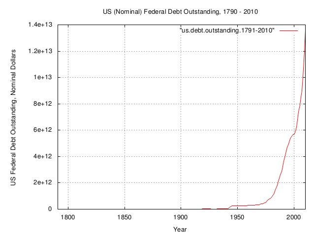
Figure I is a plot of the US nominal federal debt outstanding, 1791 through 2010.

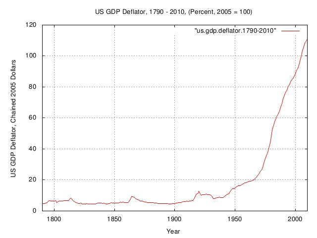
Figure II is a plot of the US GDP deflator, 1790 through 2010, in 2005 chained dollars.

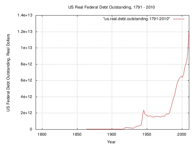
Figure III is a plot of combining the data in Figure I, which Figure II, and is the US real federal debt outstanding, 1791 through 2010, in 2005 chained dollars.

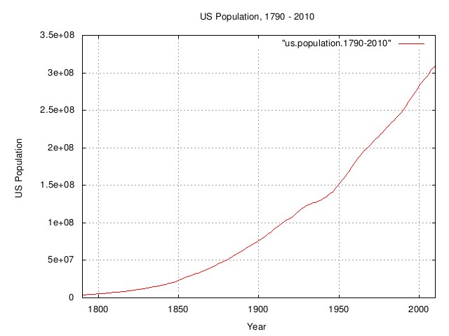
Figure IV is a plot of the US population, 1790 - 2010.

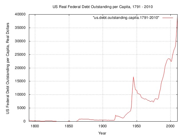
Figure V is a plot of dividing the data in Figure III, the US real federal debt outstanding, by the data in Figure IV, the US population, to obtain the US federal debt outstanding per capita, in real dollars, chained 2005.

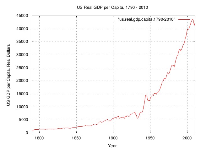
Figure VI is a plot of the US GDP per capita, chained 2005 dollars, 1790 - 2010.

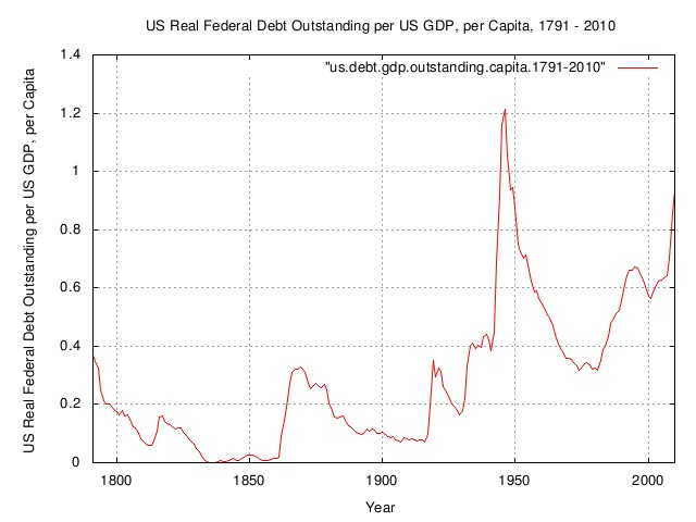
Figure VII is a plot of dividing the data in Figure V, the US federal debt outstanding per capita, in real dollars, chained 2005, by the data in Figure VI, the US GDP per capita, chained 2005 dollars, to obtain the real US federal debt outstanding per US GDP per capita, 1791 - 2010, chained 2005 dollars.

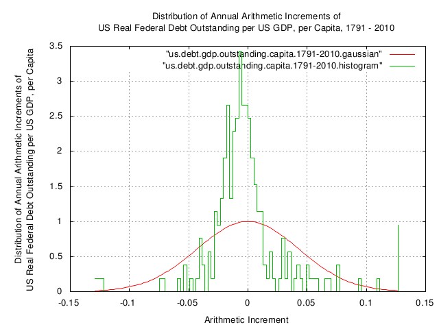
Figure VIII is a plot of the distribution of the annual arithmetic increments of the US real federal debt outstanding, per US GDP, per capita, obtained by taking the "derivative" of the data in Figure VII, the real US federal debt outstanding per US GDP per capita, 1791 - 2010, chained 2005 dollars. Notice the nearly symmetrical leptokurtosis of the increments. The Gaussian/normal LSQ of the distribution is, also, plotted.

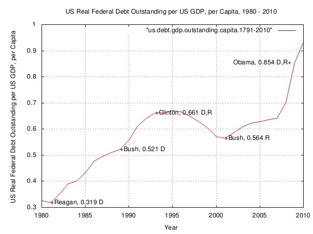
Figure IX is a plot of the real US federal debt outstanding per US GDP per capita, 1980 - 2010, chained 2005 dollars, overlayed with Presidential Administrations, and Congressional majority party affiliations.

The interpretation of the graph, for example, in 1980, everyone would have to work about a third of a year to pay off the US federal debt outstanding. In 2010, it is closer to a year.

Archive

The data presented here can be reconstructed, in its entirety, from the historical.economics.tar.gz tape archive file, which contains all data and references, thereto. The source code to all programs used in the analysis is available from the NtropiX site, tsinvest.tar.gz, and, the NdustrixX site, fractal.tar.gz, tape archive files. All use the "standard" Unix development systems of rcs(1) and make(1) to facilitate replication.

It should be noted that many of the data set sizes are pitifully small-some as few as two hundred data points, (a standard error of about 7% of the standard deviation,) and conclusions can only be regarded as circumstantial.

License

The information contained herein is private and confidential and dissemination is strictly forbidden, except under the provisions of contractual license.

THE AUTHOR PROVIDES NO WARRANTIES WHATSOEVER, EXPRESSED OR IMPLIED, INCLUDING WARRANTIES OF MERCHANTABILITY, TITLE, OR FITNESS FOR ANY PARTICULAR PURPOSE. THE AUTHOR DOES NOT WARRANT THAT USE OF THIS INFORMATION DOES NOT INFRINGE THE INTELLECTUAL PROPERTY RIGHTS OF ANY THIRD PARTY IN ANY COUNTRY.

So there.

Copyright © 1992-2016, John Conover, All Rights Reserved.

Comments, questions, and problem reports should be addressed to:

john@email.johncon.com

http://www.johncon.com/john/

http://www.johncon.com/ntropix/

http://www.johncon.com/ndustrix/

http://www.johncon.com/nformatix/

http://www.johncon.com/ndex/