The analysis of the US historical economics, 1792 through the present, will proceed with a brief description of the dynamics of the US population, followed by the US Gross Domestic Product, (GDP,) and finally, the mean US GDP per capita, which will also include a detailed analysis of the period WWII to the present, centered on the prosperity, (i.e., productivity,) "Bubble" of 1964 through 1974.

US Population

The analysis of the US population will include various eras between 1792 and the present.

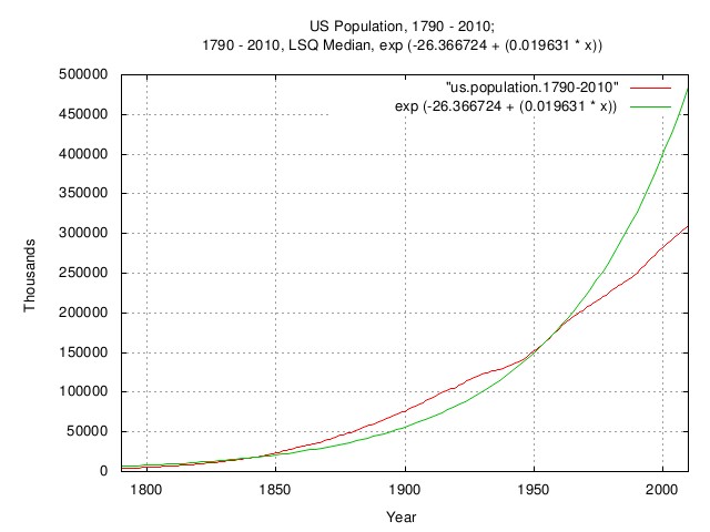
Figure I is a plot of the US population, 1790 - 2010; and the 1790 - 2010 LSQ median. (Note that median, in this case, means half of the time the empirical data is above the LSQ median, and half of the time, below.)

From 1790 to the present, the average annual increase in US population was about 2.0%, increasing to about 2.3% from 1850 through the early 1900's due to immigration. Starting in the early 1960's, the increase in US population decreased to about 1.1% annually due to family planning. Interestingly, during the Great Depression, 1929 through 1939, the birth rate decreased to about 1%, increasing to about 2.3% in the era of the post WWII "Baby Boomers."

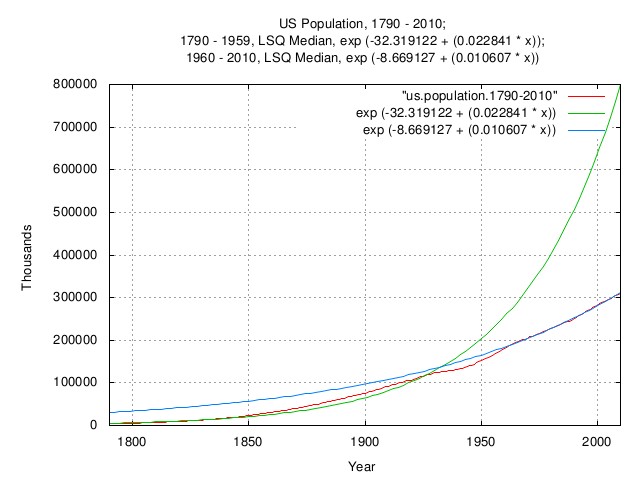
Figure II is a plot of the US population, 1790 - 2010; the 1790 - 1959 LSQ median; and the 1960 - 2010, LSQ median. (Note that median, in this case, means half of the time the empirical data is above the LSQ median, and half of the time, below.)

Note the comparison of the rate of population increase before and after the advent of family planning-the rate decreased by about a factor of 2, from about 2.2% to 1.1%, where it remains today. This was not unique to the US-it is characteristic of most of the industrialized nations: China's birth rate is near zero; Japan's slightly negative, as is Germany's, and these countries constitute over half of the world GDP.

This phenomena of decreasing birth rate has had significant consequences for GDP expansion of the industrialized nations-and related rate of government tax base increase, starting in about 1980 when the rate of increase of the work force decreased to about 1%. But note that it does not, necessarily, effect the GDP per capita, a metric of the standard of living.

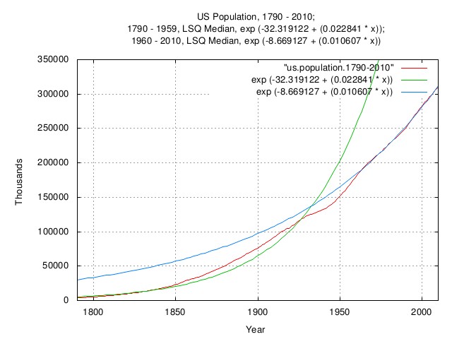
Figure III is an expanded plot of the US population, 1790 - 2010; the 1790 - 1959 LSQ median; and the 1960 - 2010, LSQ median. (Note that median, in this case, means half of the time the empirical data is above the LSQ median, and half of the time, below.) The graph range is the current population of the US.

Note that there is very little knowledge added to the study of the US population-the knowledge is quantified here.

US Gross Domestic Product

The analysis of the US GDP will include various eras between 1792 and the present.

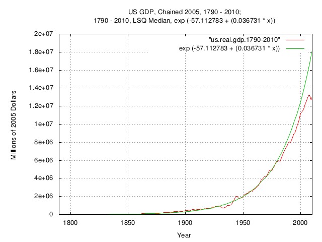
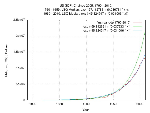
Figure IV is a plot of the US GDP, chained 2005 dollars, 1790 - 2010; and the 1790 - 2010, LSQ median. (Note that median, in this case, means half of the time the empirical data is above the LSQ median, and half of the time, below.) Historically, the US GDP's annual rate of increase averaged about 3.7%. About 2% was due to the rate of increase of the population, and, about 1.7%. due to the rate of increase in productivity.

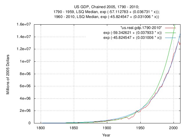
Figure V is a plot of the US GDP, chained 2005 dollars, 1790 - 2010; the 1790 - 1959, LSQ median; and the 1960 - 2010, LSQ median. (Note that median, in this case, means half of the time the empirical data is above the LSQ median, and half of the time, below.) Although, naively, it would appear that the productivity decreased post-1960. The decrease in the rate of increase of the US GDP was due to the decrease in the rate of population increase, post-1960.

Figure VI is an expanded plot of the US GDP, chained 2005 dollars, 1790 - 2010; the 1790 - 1959, LSQ median; and the 1960 - 2010, LSQ median. (Note that median, in this case, means half of the time the empirical data is above the LSQ median, and half of the time, below.) The graph range is the current US GDP.

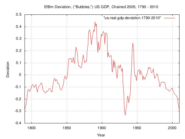
Figure VII is a plot of the EfBm deviation, ("Bubbles,") of the US GDP, chained 2005 dollars, 1790 - 2010. If the US GDP was a perfect exponential, the graph would be a straight line at zero. The graph is the deviation from the straight line at zero, i.e., the productivity "Bubbles".

The huge productivity "Bubble" of the Gilded Age, (about 1850 to 1930,) is clearly visible, (the GDP of other industrialized nations, England, Germany, and France, etc., show a similar phenomena.) The effect of the Great Depression "Bubble" decreased the US GDP by about a factor of 0.25 for about 9 years, starting in 1930, and the US GDP increased by about a factor of 0.25 in the era of WWII-this "Bubble" was mostly financed by US Government debt, (mostly held by the US population in the form of various US Government bonds; War Bonds, etc.)

The post-1960 "Bubble," was really due to a decrease in the annual population growth rate over the era.

Note that there was really no new knowledge generated here, it was just quantified for precision.

US Gross Domestic Product Per Capita

The analysis of the US GDP per capita will include various eras between 1792 and the present.

Note that both the US GDP and US population have geometric Brownian motion characteristics, and we would prefer to work with the median US GDP per capita, but annual data is not available from 1792 to the present-mandating working with the average, (or more correctly, the mean,) of the US GDP per capita, obtained by dividing the annual US GDP by the US population.

An inference is offered that the variance of the median US GDP per capita has been "reasonably" long term stable since 1792. The arguments: a perfect society would have a perfect government, (able to address economic threats expeditiously and effectively, with masterful precision, and maximization of stable growth through optimization,) meaning the median GDP per capita would increase as a perfect exponential; but real governments do not operate this way, there is a variance in the median US GDP per capita, (and it is quite similar to other industrialized countries, and has not changed much since the 1500's, the beginning of the "modern economy"); it will be shown, based on the inference that the historical variance of the median US GDP per capita has been long term stable that the dominant risk to agents in a society attempting to maximize their standard of living through increasing productivity are issues of governance-and that empirical maximization will be compared to the limitations of the Kelly Criterion.

The general analysis will proceed as follows:

• (1) Standard mean-variance analysis of the US GDP per capita; variables of interest are the average and root-mean-square of the marginal increments of the US GDP per capita, and, the variance of the marginal increments.
• (2) Log-normal analysis of the distribution of of US GDP per capita for the year 2010; variables of interest are the mode, median, and, mean of the log-normal distribution, dependent on the variables mu and rho, which we are inferring are stable since 1792, (see: Log Normal Distribution for particulars,) and the values can be obtained via LSQ analysis of the income distribution. If the inference is reasonable, then the variance of the marginal increments, obtained from 1), above, will determine how fast the ratio of median of the income distribution divided by the mode and mean, are diverging. As a verification, analyzing backwards to 1792, the values of the mode, median, and, mean, (particularly the mean,) should be representative of other societies of the era-and if they are, it is inferred that the variables are stable, and, governance is the most significant risk to the agents in a society; it would also imply that the efficiency, (or lack thereof,) of governance is stable, too.
• 3) The variance and root-mean-square of the marginal increments of the agents in a society will be more than the corresponding variables in the median of the US GDP per capita since they assume additional risk of failure in increasing their individual standard of living by attempting to increase their GDP per capita-which can be added root-mean-square to the governance risk, (assuming both are IID,) by adjusting the population by those in the work force, and the efficiency of their wagering on increasing their GDP per capita can be found via the Kelly Criterion.

In addition will be some supportive side journeys in the analysis: such as labor force participation; outlays, receipts, and debt of the US Government, on a per capita basis; and a study of the prosperity, (i.e., productivity,) "Bubble" of 1964 through 1974.

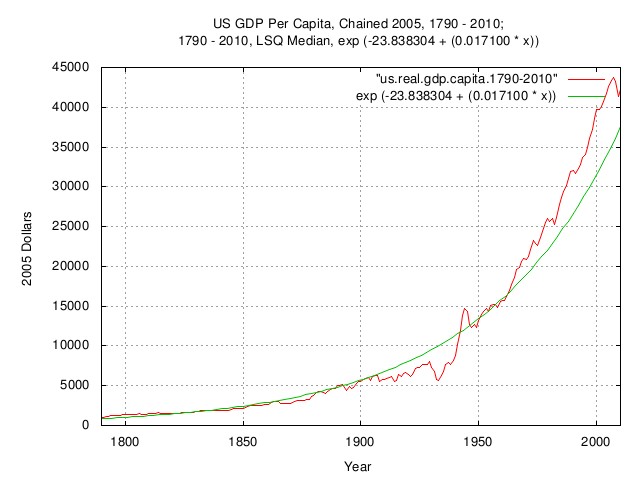
Figure VIII is a plot of the US GDP per capita, chained 2005 dollars, 1790 - 2010; and the 1790 - 2010, LSQ Median. (Note that median, in this case, means half of the time the empirical data is above the LSQ median, and half of the time, below.)

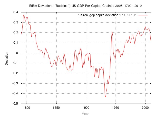
Figure IX is a plot of the EfBm deviation, ("bubbles,") of the US GDP per capita, chained 2005 dollars, 1790 - 2010. If the US GDP per capita was a perfect exponential, the graph would be a straight line at zero. The graph is the deviation from the straight line at zero, i.e., the productivity "Bubbles".

Note the comparison with Figure VII, 1950 through the present. In Figure VII, it would be naive to assume there was a decrease in prosperity since the US GDP was not growing as fast as it was previously, (remember that the decline in the US GDP growth rate was created by the decline in the post-1960 birth rate.) However, Figure IX indicates that the period from 1950 to the present was an era of unprecedented prosperity in the last two centuries.

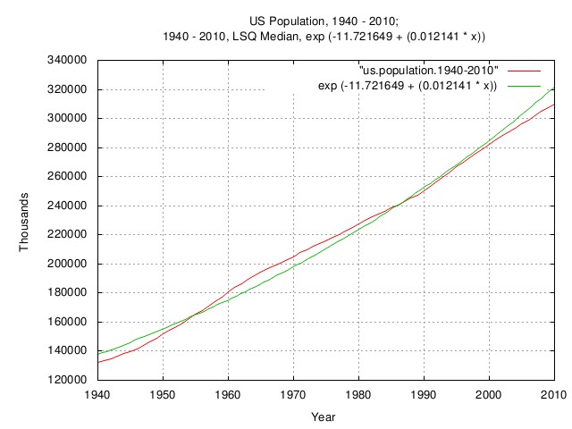
Figure X is an expanded plot of the US population, 1940 - 2010; and the 1940 - 2010, LSQ median. (Note that median, in this case, means half of the time the empirical data is above the LSQ median, and half of the time, below.)

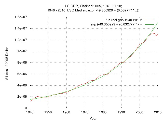
Figure XI is an expanded plot of the US GDP, chained 2005 dollars, 1940 - 2010; and the 1940 - 2010, LSQ median. (Note that median, in this case, means half of the time the empirical data is above the LSQ median, and half of the time, below.)

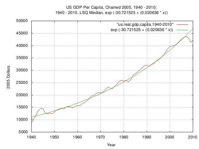
Figure XII is an expanded plot of the US GDP per capita, chained 2005 dollars, 1940 - 2010; and the 1940 - 2010, LSQ median. (Note that median, in this case, means half of the time the empirical data is above the LSQ median, and half of the time, below.)

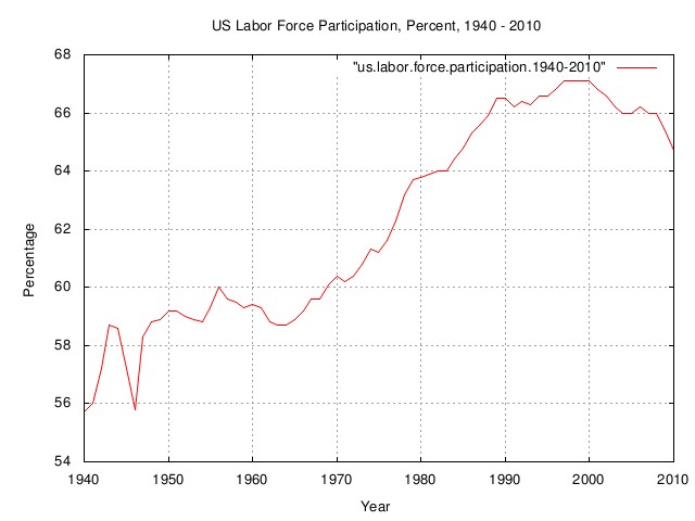
Figure XIII is a plot of the US labor force participation, percent, 1940 - 2010. There is a lot of dynamics shown in this graph. From the late 1940's through the early 1960's, the "Baby Boomers" were growing up, and their count was included in the population; but they were not contributing to the US productivity, (other than consumption.) Starting in about 1964, they moved into the workplace and contributed to the US GDP, increasing, (quite rapidly,) the GDP per capita-for about five years. This was followed by an influx of females into the workplace, for about another 5 years, increasing the GDP per capita, (remember that the birth rate had been in decline since the early 1960's,) so much so that almost 2/3 of the households were dual-income. The consequence of these dynamics made a significant contribution to the prosperity, (i.e., productivity,) "Bubble" of 1964 through 1974. A similar scenario occurred in other industrialize nations over the period, too.

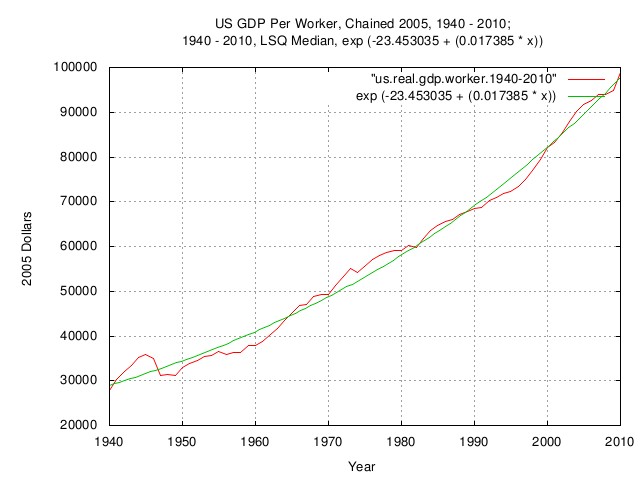
Figure XIV is a plot of the US GDP per worker, chained 2005 dollars, 1940 - 2010; and the 1940 - 2010, LSQ Median. (Note that median, in this case, means half of the time the empirical data is above the LSQ median, and half of the time, below.) Using the data in Figure XIII, the mean US GDP per worker can be calculated. It is important to note that the productivity of the US worker increased at a rate of almost 1.8% a year since WWII, meaning the standard of living increased about the same. This is an important number, and has remained nearly constant in the US at about 1.7% from 1792, and about 1.6% for the world GDP since the early 1500's, the beginning of the "modern economy." It is not clear why this number is ubiquitous.

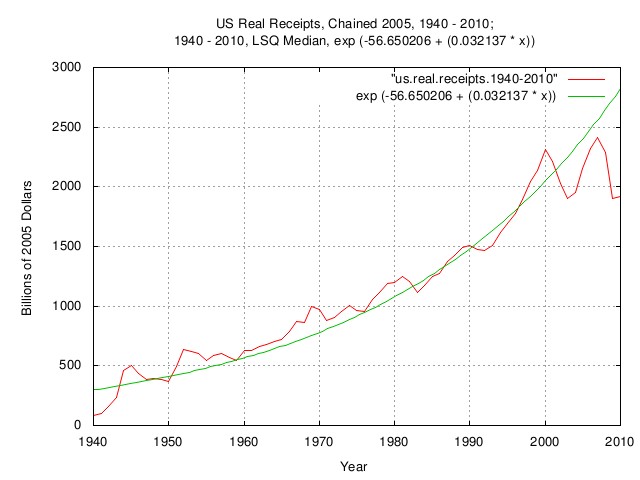
Figure XV is a plot of the US real receipts, chained 2005 dollars, 1940 - 2010; and the 1940 - 2010, LSQ median. (Note that median, in this case, means half of the time the empirical data is above the LSQ median, and half of the time, below.) The US Government's response to the prosperity, (i.e., productivity,) "Bubble" of 1964 through 1974 is shown, as is the decline in the tax-base in the early 1980's due to the post-1960 decline in birth rate.

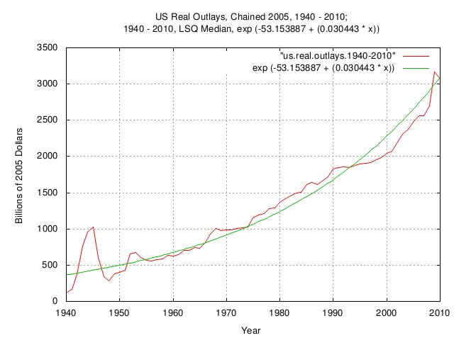
Figure XVI is a plot of the US real outlays, chained 2005 dollars, 1940 - 2010; and the 1940 - 2010, LSQ median. (Note that median, in this case, means half of the time the empirical data is above the LSQ median, and half of the time, below.) Note the decline in outlays starting in the early 1990's.

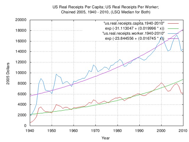
Figure XVII is a plot of the US real receipts per capita; the US real receipts per worker; both chained 2005 dollars, 1940 - 2010; and the LSQ median for both. (Note that median, in this case, means half of the time the empirical data is above the LSQ median, and half of the time, below.) The US Government's tax-base income during the prosperity, (i.e., productivity,) "Bubble" of 1964 through 1974 is shown, as is the decline starting in about 2000.

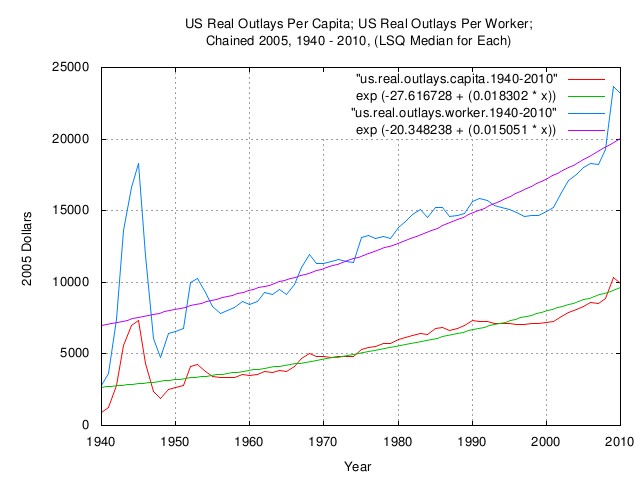
Figure XVIII is a plot of the US real outlays per capita; the US real outlays per worker; both chained 2005 dollars, 1940 - 2010; and the LSQ median for each. (Note that median, in this case, means half of the time the empirical data is above the LSQ median, and half of the time, below.)

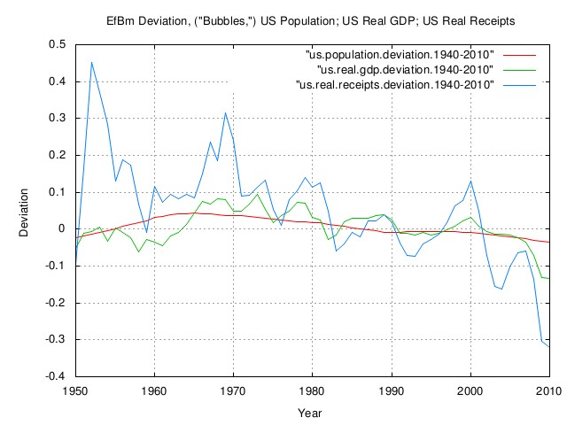
Figure XIX is a plot of the EfBm deviation, ("bubbles,") of the US population; the US real GDP; and the US real receipts; all 1940 - 2010.

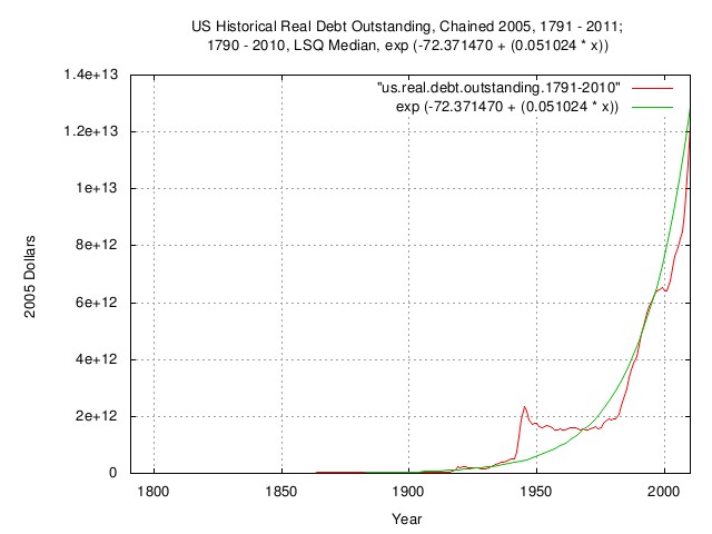
Figure XX is a plot of the US historical real debt outstanding, chained 2005 dollars, 1791 - 2011; and the 1790 - 2010, LSQ median. (Note that median, in this case, means half of the time the empirical data is above the LSQ median, and half of the time, below.) Note accruing of debt following the prosperity, (i.e., productivity,) "Bubble" of 1964 through 1974.

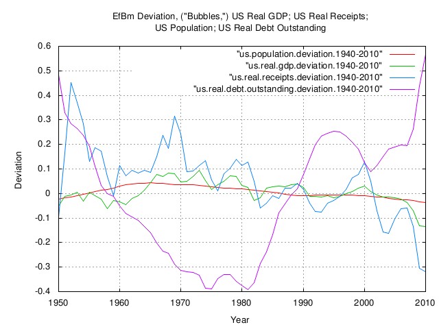
Figure XXI is a plot of the EfBm deviation, ("bubbles,") of the US real GDP; the US real receipts; the US population; and the US real debt outstanding. Note that the the US real debt outstanding is shown for methodological completeness. Debt can not have geometric Brownian motion characteristics since debt can be zero, or negative, (i.e., balanced, or a surplus, respectively.) Debt must be analyzed differently since it has arithmetic Brownian motion characteristics.

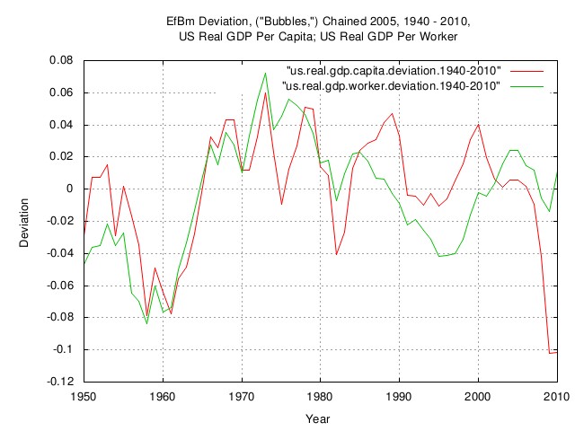
Figure XXII is a plot of the EfBm deviation, ("Bubbles,") chained 2005 dollars, 1940 - 2010, of the US real GDP per capita; and the US real GDP per worker. The prosperity, (i.e., productivity,) "Bubble" of 1964 through 1974 can clearly be seen-increasing about 7% a year, or between 1964 and 1974, it almost doubled. At the current rate of 1.7%, it would double in 41 years. A similar scenario is extant for the other industrialized nations, too.

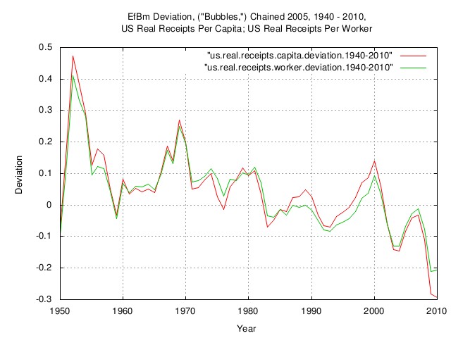
Figure XXIII is a plot of the EfBm deviation, ("Bubbles,") chained 2005 dollars, 1940 - 2010, of the US real receipts per capita; and the US real receipts per worker. Note the size of the negative "Bubble" starting in about 2000.

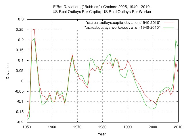
Figure XXIV is a plot of the EfBm deviation, ("Bubbles,") chained 2005 dollars, 1940 - 2010, of the US real outlays per capita; and the US real outlays per worker.

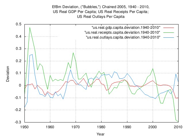
Figure XXV is a plot of the EfBm deviation, ("Bubbles,") chained 2005 dollars, 1940 - 2010, of the US real GDP per capita; the US real receipts per capita; and the US real outlays per capita.

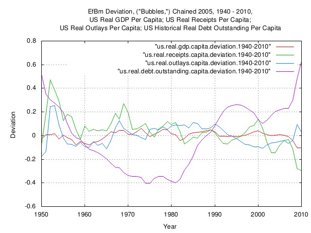
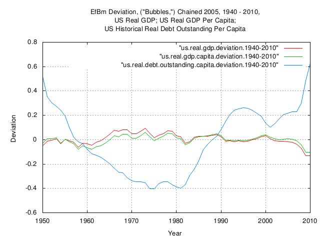
Figure XXVI is a plot of the EfBm deviation, ("bubbles,") chained 2005 dollars, 1940 - 2010, of the US real GDP per capita; the US real receipts per capita; the US real outlays per capita; and the US historical real debt outstanding per capita. Note that the the US real debt outstanding is shown for methodological completeness. Debt can not have geometric Brownian motion characteristics since debt can be zero, or negative, (i.e., balanced, or a surplus, respectively.) Debt must be analyzed differently since it has arithmetic Brownian motion characteristics.

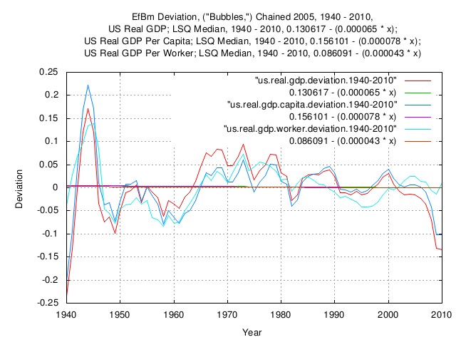
Figure XXVII is a plot of the EfBm deviation, ("bubbles,") chained 2005 dollars, 1940 - 2010, of the US real GDP; the US real GDP per capita; the US real GDP per worker, and LSQ medians for all three. (Note that median, in this case, means half of the time the empirical data is above the LSQ median, and half of the time, below.) Note that the time horizon for the LSQ of data 1940 - 2010, the LSQ median is zero. If one basis an economic comparison on data starting in 1964, the prosperity, (i.e., productivity,) "Bubble" of 1964 through 1974, one will interpret the data quite differently, as shown in the next figure, Figure XXVIII.

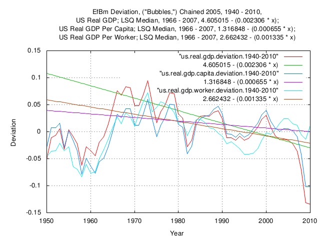
Figure XXVIII is an expanded plot of the EfBm deviation, ("bubbles,") chained 2005 dollars, 1940 - 2010, of the US real GDP; the US real GDP per capita; the US real GDP per worker, and 1966 - 2007 LSQ medians for all three. (Note that median, in this case, means half of the time the empirical data is above the LSQ median, and half of the time, below.) The expansion is centered around the mid 1960's through late 1970's prosperity, (productivity,) "bubble, which is clearly visible. Note that the time horizon for the LSQs of data 1966 - 2010, the LSQ medians have a negative tilt. If one bases an economic interpretation on data starting in 1966, one would interpret the data quite differently-as a long term decline in the US economy, as opposed to the previous graph, Figure XXVII, which uses the same data, but the LSQ's include data back to 1940. (The point is that people, naturally, compare the current era with eras of the past, and can draw erroneous interpretations due to the time horizons they are comparing-in the case of this graph, the comparison era was the mid 1960's through late 1970's prosperity, (productivity,) "bubble," alas which did not last.)

Figure XXIX is a plot of the EfBm deviation, ("bubbles,") chained 2005 dollars, 1940 - 2010, of the US real GDP; the US real GDP per capita; and the US historical real debt outstanding per capita. Note that the the US real debt outstanding is shown for methodological completeness. Debt can not have geometric Brownian motion characteristics since debt can be zero, or negative, (i.e., balanced, or a surplus, respectively.) Debt must be analyzed differently since it has arithmetic Brownian motion characteristics.

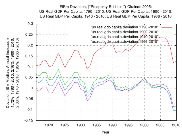
Figure XXX is a plot of the EfBm deviation, ("prosperity bubbles,") chained 2005 dollars, of the US real GDP per capita, 1790 - 2010; the US real GDP per capita, 1900 - 2010; the US Real GDP per capita, 1940 - 2010; and the US real GDP per capita, 1966 - 2010. Note that from 1792 through about 1950, much of the US economy was rural agricultural. Comparing this with the current industrialized era, the US economy is in a long term prosperity "bubble." However, comparing the current era with more recent eras indicates a similarity, with peak-to-peak "bubbles" in about a 7% band of each other.

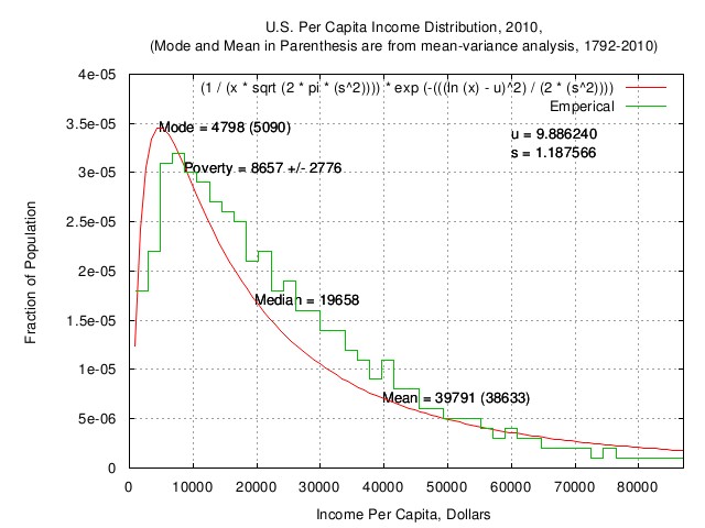
Figure XXXI is a plot of the US per capita income distribution, 2010, (mode and mean in parenthesis are from mean-variance analysis, 1792-2010.) From the us.income.distribution.README.txt worksheet it would appear that the the US per capita income, (implying US per capita GDP through Production approach and Income approach, equalities,) 2010, is consistent with the mean, (time average,) and root-mean-square of the marginal increments of US GDP from 1792 through 2010, i.e.,the inference offered that the variance of the median US GDP per capita has been "reasonably" long term stable since 1792, and, issues of governence being the largest risk factor in the growth of the US GDP per capita, meaning increasing "prosperity.".

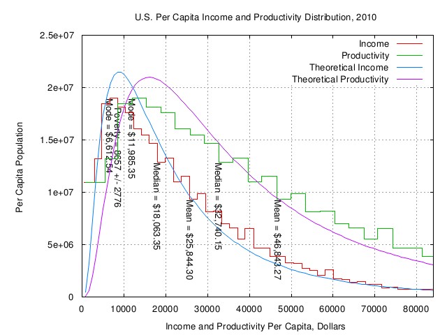
Figure XXXII is a plot of the US per capita income and productivity distribution, 2010. This graph is different from the previous graph in that the household data is converted to US per capita income and productivity. The worksheet is an emacs/gnuplot script file, us.income.distribution.gp.txt.

The objective being to develop an analysis of the efficiencies of the ensemble average of the US GDP per worker, i.e., those that actually generate the US GDP, (as opposed to the US GDP per capita-about half of which do not contribute to the productivity, other than consumption.)

In a nutshell, what is being looked for is the efficiences of the gambling at increasing the individual prosperity, (i.e., US GDP per worker,) in the US GDP that has geometric Brownian motion characteristics. In the long run, luck will average out for almost all of the workers-the successful will understand how to exploit the luck, while at the same time minimizing risk to their prosperity, i.e., optimize the long term growth in their prosperity. But that can be determined by comparing their metrics with the Kelly Criterion.

In terms of the real GDP, the development of the data is in the work files, us.real.gdp.capita.1790-2010.README.txt and, us.real.gdp.distribution.2010.txt.

Excerpts for the real GDP:

• An individual's risk assessment to the mean real US GDP per capita, (i.e., real standard of living,) is dominated by issues of governance by about a factor of two. In the case of the annual mean real US GDP per capita, the wagering on innovation risk is about 2.7%, (which is about 4.3% of optimal,) but the equivalent wagering on governance risk is 4.7%, (which is about 12.2% of optimal,) nearing twice as much, (if it is assumed that the affects of governance risk affect the mean and median of the mean real US GDP per capita about the same, since governance risk affects all, or nearly all, of the population.)
• ... individuals who are expanding the annual mean real US GDP per capita, at an annual exponential rate of 1.016, are doing so at a 27.0% efficiency, relative to the limitations of the Kelly Criterion, which places a maximum annual exponential rate limit of 1.060 on the growth of the mean real US GDP per capita. The fractional Kelly Criterion is about 15.2%.
• Note that the World's real mean GDP annual growth per capita has not changed since the early 1800's, (measured in 1990 International Dollars, records prior to 1850 removed,) ... which is about the same time [as the US at 1650,], (see: ../historical/world.gdp.capita.10000BCE-2010,) [which is when] the modern era of civilization started; the world GDP per capita was nearly constant from the age of flint until 1600, when the rate of annual increases in the mean world real GDP per capita increased from unity to about 1.017, and has remained constant since the 1600's. Similarly, for the mean real US GDP per capita.

In terms of the nominal GDP, the development of the data is in the work files, us.nominal.gdp.capita.1790-2010.README.txt and, us.nominal.gdp.distribution.2010.txt.

Excerpts for the nominal GDP:

• An individual's risk assessment to the mean nominal US GDP per capita, (i.e., nominal standard of living,) is dominated by issues of governance by about a factor of two. In the case of the annual mean nominal US GDP per capita, the wagering on innovation risk is about 3.7%, (which is about 4.5% of optimal,) but the equivalent governance risk is 8.6%, (which is about 21.1% of optimal,) slightly more than twice as much, (if it is assumed that the affects of governance risk affect the mean and median of the mean nominal US GDP per capita about the same, since governance risk affects all, or nearly all, of the population.)
• ... individuals who are expanding the annual mean nominal US GDP per capita, at an annual exponential rate of 1.027, are doing so at a 42.1% efficiency, relative to the limitations of the Kelly Criterion, which places a maximum annual exponential rate limit of 1.063 on the growth of the mean nominal US GDP per capita. The fractional Kelly Criterion is about 24.9%.
• Note that the World's real mean GDP annual growth per capita has not changed since the early 1800's, (measured in 1990 International Dollars, records prior to 1850 removed,) ... which is about the same time [as the US at 1650,], (see: ../historical/world.gdp.capita.10000BCE-2010,) [which is when] the modern era of civilization started; the world GDP per capita was nearly constant from the age of flint until 1600, when the rate of annual increases in the mean world real GDP per capita increased from unity to about 1.017, and has remained constant since the 1600's. Similarly, for the mean real US GDP per capita.

It is interesting that the US worker seems to be wagering on increasing prosperity based more on the value of the nominal dollar, (possibly since debt is denominated and payed off in nominal dollars,) instead of the real dollar, and is doing so at 25% efficiency, relative to the optimal Kelly Criterion, (i.e., fractional Kelly Criterion, which possibly indicates risk-aversion: perhaps due to persistence of economic conditions from one year to the next, instead of being IID, as assumed in this analysis; a Leptokurtic/Black Swan distribution of the marginal increments of the US nominal GDP; etc.) Interestingly, the contemporary empirical value of fractional Kelly Criterion used by Hedge Funds to reduce the risk of short term Drawdowns, is commensurate with this value, (Thorp, et al.) The dominant assessment of risk to enhancement of prosperity by the US worker seems to be concerns of governance, (as opposed to personal failure, i.e., creating new ideas that don't work out,) by about a factor of two. These variable values seem to have been relatively consistent for over two centuries, and are consistent with the variable values of the world GDP for three or four centuries, (i.e., the "modern economy.") If it is assumed that an increase in GDP per capita is created by a corresponding proportional increase in knowledge, then the time-to-double knowledge would be 0.7 / ln (1.017) ~ 40 years over these centuries, which is reasonably consistent with inferential estimates, (Fuller, et al.)

                         rms^2
                 M = 1 - ----- ......................................(B-1.35)
                          avg

               

Archive

The data presented here can be reconstructed, in its entirety, from the historical.economics.tar.gz tape archive file, which contains all data and references, thereto. The source code to all programs used in the analysis is available from the NtropiX site, tsinvest.tar.gz, and, the NdustrixX site, fractal.tar.gz, tape archive files. All use the "standard" Unix development systems of rcs(1) and make(1) to facilitate replication.

It should be noted that many of the data set sizes are pitifully small-some as few as two hundred data points, (a standard error of about 7% of the standard deviation,) and conclusions can only be regarded as circumstantial.

License

The information contained herein is private and confidential and dissemination is strictly forbidden, except under the provisions of contractual license.

THE AUTHOR PROVIDES NO WARRANTIES WHATSOEVER, EXPRESSED OR IMPLIED, INCLUDING WARRANTIES OF MERCHANTABILITY, TITLE, OR FITNESS FOR ANY PARTICULAR PURPOSE. THE AUTHOR DOES NOT WARRANT THAT USE OF THIS INFORMATION DOES NOT INFRINGE THE INTELLECTUAL PROPERTY RIGHTS OF ANY THIRD PARTY IN ANY COUNTRY.

So there.

Copyright © 1992-2017, John Conover, All Rights Reserved.

Comments, questions, and problem reports should be addressed to:

john@email.johncon.com

http://www.johncon.com/john/

http://www.johncon.com/ntropix/

http://www.johncon.com/ndustrix/

http://www.johncon.com/nformatix/

http://www.johncon.com/ndex/