|
From: John Conover <john@email.johncon.com>
Subject: Quantitative Analysis of Non-Linear High Entropy Economic Systems III
Date: 14 Feb 2002 07:38:46 -0000
As mentioned in Section I and Section II, much of applied economics has to address non-linear high entropy systems-those systems characterized by random fluctuations over time-such as net wealth, equity prices, gross domestic product, industrial markets, etc.
The characteristic dynamics, over time, of non-linear high entropy systems evolve into log-normal distributions requiring suitable methodologies for analysis.
Note: the C source code to all programs used are available from the NtropiX Utilities page, or, the NdustriX Utilities page, and are distributed under License.
It is frequently expedient to convert a non-linear high entropy economic system's characteristics to the Brownian motion/random walk fractal equivalent described in Section II to analyze the system's dynamics. A non-linear high entropy time series can be converted to a Brownian motion/random walk fractal time series by simply taking the logarithm of time series:
tsmath -l file > file.brownian.motion
where file is the non-linear
high entropy time series input file, and
file.brownian.motion is the
Brownian motion/random walk equivalent time series output file.
Analyzing the time series for a non-linear high entropy system:
    tsfraction file | tsrms -p
    tsfraction file | tsavg -p
will print the value of the root-mean-square and average of the
time series' marginal increments, rms,
and, avg, respectively. The probability
of an up movement, P, in the time series
is:
        avg
        --- + 1
        rms
    P = ------- ........................................(1.24)
           2
from Section
I, and the exponential marginal gain per unit time,
g, is:
                 P          (1 - P)
    g = (1 + rms)  (1 - rms)        ....................(1.20)
After t many time intervals, on
average, the non-linear high entropy time series' value would have
increased by a factor of g^t.
Analyzing the Brownian motion/random walk equivalent of the non-linear high entropy system's time series:
    tsderivative file.brownian | tsrms -p
    tsderivative file.brownian | tsavg -p
or:
    tsmath -l file | tsderivative | tsrms -p
    tsmath -l file | tsderivative | tsavg -p
will print the root-mean-square and average of the marginal
increments of the Brownian motion/random walk equivalent time series,
rms, and,
avg, respectively.
After t many time intervals, on
average, the Brownian motion/random walk equivalent time series' value
would have increased by a factor of avg *
t.
The reason for working with the Brownian motion/random walk equivalent time series is that the dynamics are intuitive and mathematically expedient.
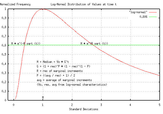
For the Brownian motion/random walk equivalent, the value of the
median, (which is the same as the mean for a random walk,) increases
by avg * t in
t many time units-meaning that half of
the time, the median value will be greater than avg *
t, and half less.
For the Brownian motion/random walk equivalent, the distribution
around the median increases by rms * sqrt
(t) in t many time
units-meaning that for one deviation, 84.134474607%, of the time, the
value will be less than rms * sqrt (t),
and 84.134474607% of the time greater than -rms * sqrt
(t).
|
As a side bar, this is an intuitive result. The
"prescription" for making a Brownian motion/random walk fractal
is to start with an initial value, and add a random number with
a normal/Gaussian distribution. Then add another random number,
and another, and so on, one each for each time unit,
Normal/Gaussian distributions add root-mean-square, so it
would be expected that the deviation of the Brownian
motion/random walk around the median increases by a factor of
|
For the Brownian motion/random walk equivalent, the cumulative
probability of the duration between crossings of the median value, in
t many time units, is erf
(1 / sqrt (t)), meaning that once its value has
crossed the median, the probability that it will not cross the median
again for at least t many time units is
equal to erf (1 / sqrt (t)).
|
As a side bar, The term |
For the Brownian motion/random walk equivalent, the two equations:
rms * sqrt (t) .....................................(3.1)
erf (1 / sqrt (t)) .................................(3.2)
are useful for analyzing the probabilities of the
magnitude and duration, respectively, of
bubbles in high entropy economic systems; the latter can be
used as the probability that, by serendipity, an analysis was made of
a data set acquired during a bubble, (like the dot-com
bubble, for example.) The technique is a form of statistical
estimation, but used in an unconventional way-for analyzing
economic bubbles, (note the isomorphism between the
convergence of Bernoulli
P Trials and economic bubbles). Multiplying Equation
(1.24) from Section
I by 1 - erf (1 / sqrt (t)):
avg
--- + 1
rms
P = ------- * (1 - erf (1 / sqrt (t))) .............(3.3)
2
would give the average probability of an up movement in a
non-linear high entropy system, compensated for data set size, or
measurement time interval. For example, for the metric P
= 0.59, measured over t =
50 daily closes of an equity price, or
erf (1 / sqrt (50)) = 0.840691, the
effective probability of an up movement in the marginal
increments would be 0.840691 * 0.59 =
0.49600769, which is not a choice as an investment
opportunity-more time would be required for the measurement of
P. This methodology can be extended; see
the documentation
for the tsshannoneffective
program for the particulars of the numerical methods involved. The
technique allows economic systems with different characteristics, and
dissimilar data set sizes, to be optimized by sorting on the
effective probability of an up movement in the marginal
increments.
|
As a side bar, many of the dot-com companies were
running a probability of an up movement, Probably not. The problem is more complicated, however, and the accuracy of
both the average, showing that a calendar quarter of daily data is far from adequate. In point of fact, the break even chance for such an investment: requires about 7 calendar quarters of daily data. To be favored over the typical stock on the US exchanges: about 3 calendar years of data supporting In some sense, the technique is a utilization of the null
hypothesis. By serendipity, a Brownian motion/random walk
data set with |
Mapping back and fourth between the dynamic characteristics of non-linear high entropy system and its Brownian motion/random walk equivalent is straight forward-take the logarithm of the data to get to the random walk model, and exponentiate to get back.
|
|
Figure I shows the log-normal characteristics of the dynamics of a non-linear high entropy system, and how the characteristics map to its Brownian motion/random walk equivalent.
|
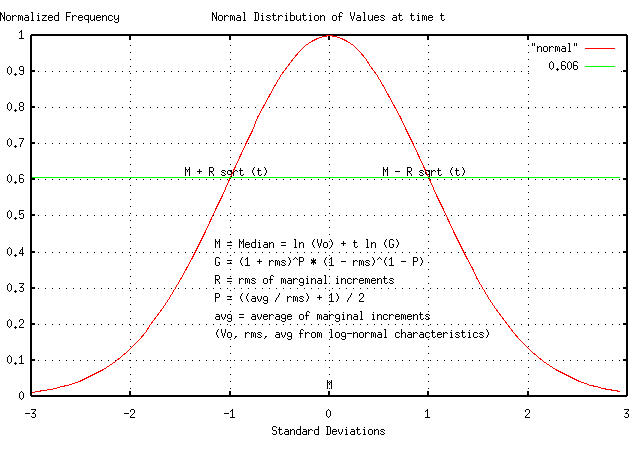
Figure II shows the Brownian motion/random walk equivalent, and how the dynamic characteristics map back into log-normal non-linear high entropy dynamics.
Reiterating the important equations for the characteristic dynamics, over time, of high entropy economic systems, the probabilities of the magnitude and duration, respectively, of bubbles in the high entropy economic system Brownian motion/random walk equivalent time series:
rms * sqrt (t) .....................................(3.1)
erf (1 / sqrt (t)) .................................(3.2)
and the probability of an up movement in a high entropy economic system, compensated for data set size, or measurement time interval in the Brownian motion/random walk equivalent time series:
        avg
        --- + 1
        rms
    P = ------- * (1 - erf (1 / sqrt (t))) .............(3.3)
           2
The file
djia.jan.02.1900-feb.15.2002
contains the time series history of the daily closes for the DJIA,
from January 2, 1900, through, February 15, 2002, (27,938 trading
days,) inclusive. The DJIA's initial value, on January 2, 1900, was
68.13.
Analysis:
    tsfraction djia.jan.02.1900-feb.15.2002 | tsrms -p
    0.010972

    tsfraction djia.jan.02.1900-feb.15.2002 | tsavg -p
    0.000239

    wc djia.jan.02.1900-feb.15.2002
    27938   55880  445031 djia.jan.02.1900-feb.15.2002
where, from Equation (1.24):
        avg       0.000239
        --- + 1   -------- + 1
        rms       0.010972
    P = ------- = ------------ = 0.51089136 ............(3.5)
           2           2
in Section I.
where P is a likelihood of an up
movement in the DJIA, and, for simulating the DJIA, the file,
sim contains a single
record:
DJIA, p = 0.51089136, f = 0.010972, i = 68.13
and the exponential marginal gain per unit time,
g, is:
                 P          (1 - P)
    g = (1 + rms)  (1 - rms)


                      0.51089136
      = (1 + 0.010972)

                        1 - 0.51089136
        * (1 + 0.010972)

      = 1.00017882956 ..................................(3.6)
and, using the tsinvestsim
program:
tsinvestsim sim 27938 > tsinvestsim.djia.jan.02.1900-feb.15.2002
The cumulative probability of the duration between the DJIA's value crossing its median value, and its simulation:
    tsmath -l djia.jan.02.1900-feb.15.2002 | tslsq -o | \
        tsrunlength | cut -f1,7 > djia.jan.02.1900-feb.15.2002.runlength

    tsmath -l tsinvestsim.djia.jan.02.1900-feb.15.2002 | tslsq -o | \
        tsrunlength | cut -f1,7 > tsinvestsim.djia.jan.02.1900-feb.15.2002.runlength
|
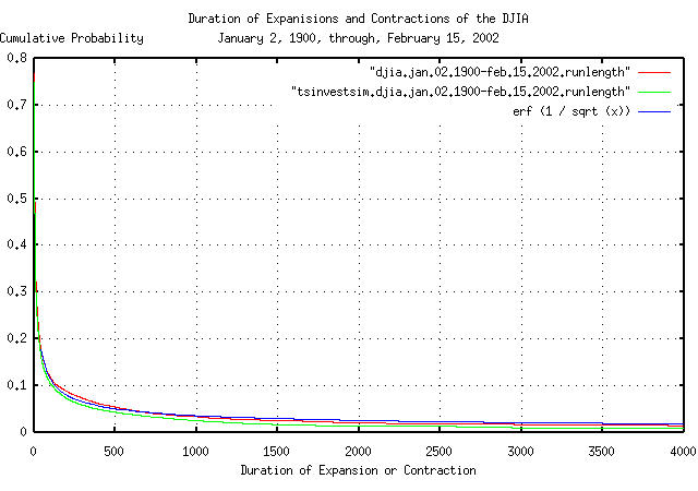
Figure III is a plot of the cumulative probability of the duration
of the expansions and contractions of the DJIA, and its simulation,
with the theoretical value, erf (1 / sqrt
(t)). The frequency of durations of up to 4,000
trading days, (about 16 calendar years,) are shown.
|
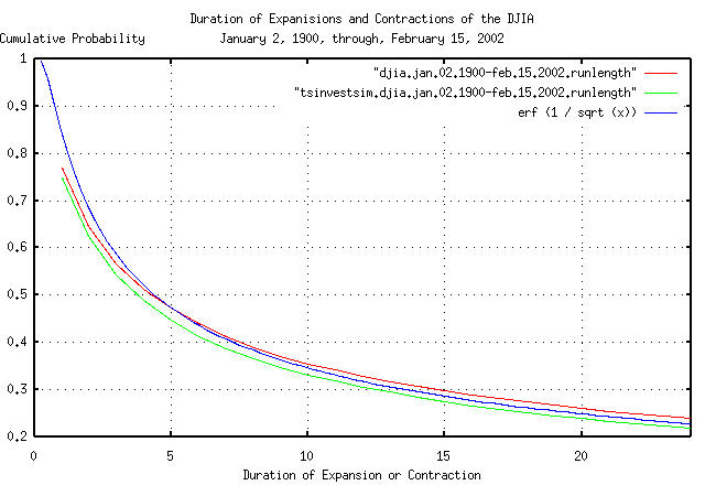
Figure IV is a plot of the cumulative probability of the duration
of the expansions and contractions of the DJIA, and its simulation,
with the theoretical value, erf (1 / sqrt
(t)) from Figure III. The frequency of durations of up
to 30 trading days, (about one and a half calendar months,) is shown
for clarity. 4.396233 days is the median value for an expansion or
contraction for daily data-half of the expansions, or contractions,
last less than 4.4 trading days, half more, (where erf
(1 / sqrt (4.396233)) = 0.5.)
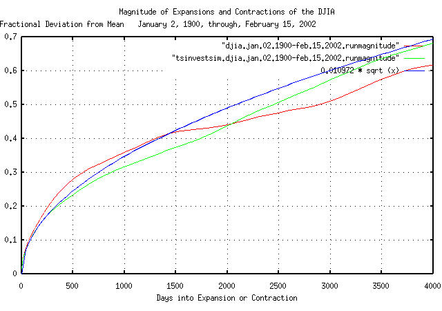
The deviation from the mean of the expansions and contractions of the DJIA, and its simulation:
tsmath -l djia.jan.02.1900-feb.15.2002 | tslsq -o | \
tsrunmagnitude > djia.jan.02.1900-feb.15.2002.runmagnitude
tsmath -l tsinvestsim.djia.jan.02.1900-feb.15.2002 | tslsq -o | \
tsrunmagnitude > tsinvestsim.djia.jan.02.1900-feb.15.2002.runmagnitude
|
Figure V is a plot of the deviation from the mean of the expansions
and contractions of the DJIA, and its simulation, with the theoretical
value of 0.010972 * sqrt (t). The
deviation of expansions, or contractions, of up to 4,000 trading days,
(about 16 calendar years,) are shown.
|
As a side bar, the forensics of the 1929 stock market crash are interesting. On September 3, 1929, the DJIA closed at a record high of 381.17. The DJIA deteriorated to 298.97 by October 26, 1929, and on October 28, it declined 12.8207%, closing at 260.64-which was the greatest single day percentage loss in the history of the DJIA until October 19, 1989 when it lost 22.6105% in a single day. But it was not over. The next trading day, October 29, 1929, it lost another 11.7288% to close at 230.07. By December 7, 1929, the DJIA had increased back to 263.46 and drifted positive to close at 294.43 on April 12, 1930. Then, it constantly deteriorated for 667 trading days to close at a low of 41.22 on July 8, 1932-which was its record low for the twentieth century. The DJIA did not regain its pre-crash value until November 23, 1954, when it closed at 382.74-a quarter of a century after the 1929 stock market crash. It took 843 trading days from its September 3, 1929 high of 381.17 to lose 89.1859275% of its value and close at its low of 41.22 on July 8, 1932. What are the chances of an economic catastrophe of such magnitude happening again? Working with the Brownian motion/random walk equivalent of the DJIA: where Equation (3.7) is a bit difficult to use, and there is a useful approximation in Appendix I What are the chances of an economic catastrophe of such duration happening again? or there is about a 1.4% chance of the DJIA being below its median value for 25 years, or 6,325 business days of 253 business days per year. The magnitude of the decline in equity values that occurred in the Great Depression of the 1930's was a very rare event. However, the duration of the decline was not. What's the chances of economic system, like the DJIA, decreasing in value by at least 47%, in a calendar year of 253 business days? where As a concluding remark in this side bar, the methodology used
assumes that equity markets are efficient in the sense of Eugene
Fama's Efficient
Market Hypothesis, as a mathematical expediency. However,
not everyone in the market responds instantaneously to new
market information. There is a very slight short term
persistence in market dynamics in response to market
information-about 57%, measured on the daily closes of the DJIA
with the The leptokurtosis means that the standard deviation and mean
can not be used, (since they diverge,) and one must work with
the median and interquartile ranges. However, for very short
term persistence, (i.e., the market is close to being
efficient,) the deviation of catastrophic events can be
approximated with the standard deviation calculated by using
(As a sanity check, if it is assumed that the DJIA is a typical equity index, and there are about 200 such indices on the planet, one each for each of the 200 countries, then we would expect to see the equivalent of a 1929 crash in about 33 of the country's indices in a century-which is about what was seen in the Twentieth Century's worst crashes-the 1929 US market catastrophe, the worst of the Asian Contagion, Latin American economic melt down, USSR collapse, etc.) |
The file us.gdp.1930-1995
contains the time series history of the US annual GDP from 1930,
through, 1995, (66 years,) inclusive. The data is from the 1997 US Federal Budget, and
references FED data.
The file
us.gdp.q1.1979-q4.1996 contains
the time series history of the US quarterly GDP from Q1, 1979,
through, Q4, 1996, (72 quarters,) inclusive. The data is from the US
DOC, file QIGNGDPK, and references FED data, and is seasonally
adjusted annual rate, (SAAR.)
Both data sets are pitifully small, and SAAR data is not appropriate for analyzing the dynamic characteristics of a time series. In addition, it appears that the quarterly data was a running average of four quarters.
Analysis:
The cumulative probability of the duration between the US GDP's values crossing its median value:
wc us.gdp.1930-1995
66 132 924 us.gdp.1930-1995
tsshannoneffective -e dummy dummy 66
erf (1 / sqrt (66)) = 0.138926, 1 - erf (1 / sqrt (66)) = 0.861074
tsmath -l us.gdp.1930-1995 | tslsq -o | tsrunlength | \
cut -f1,7 | tsmath -a 0.138926 > 'us.gdp.1930-1995.runlength+0.138926'
wc us.gdp.q1.1979-q4.1996
72 72 648 us.gdp.q1.1979-q4.1996
tsshannoneffective -e dummy dummy 72
erf (1 / sqrt (72)) = 0.132635, 1 - erf (1 / sqrt (72)) = 0.867365
tsmath -l us.gdp.q1.1979-q4.1996 | tslsq -o | tsrunlength | \
cut -f1,7 | tsmath -a 0.132635 > 'us.gdp.q1.1979-q4.1996.runlength+0.132635'
where the entire cumulative distribution was missing past 66 years
for the annual data, and 72 quarters for the quarterly data-the
theoretical distribution past these values, from the tsshannoneffective
program, was added to the emperically derived distributions.
|
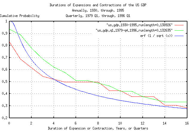
Figure VI is a plot of the cumulative probability of the duration
of the annual and quarterly expansions and contractions of the US GDP,
with the theoretical value, erf (1 / sqrt
(t)). Note that the median time the US GDP is above,
or below, its median value is 4.396233 years, since 0.5
= erf (1 / sqrt (4.396233), i.e., the median business
cycle is 4.4 years-half of the business cycles last less that 4.4
calendar years, half more. Likewise for calendar quarters, which
implies fractal characteristics.
The deviation from the mean of the expansions and contractions of the US GDP:
tsmath -l us.gdp.1930-1995 | tslsq -o | tsderivative | tsrms -p
0.069817
tsmath -l us.gdp.1930-1995 | tslsq -o | \
tsrunmagnitude > us.gdp.1930-1995.runmagnitude
tsmath -l us.gdp.q1.1979-q4.1996 | tslsq -o | tsderivative | tsrms -p
0.007833
tsmath -l us.gdp.q1.1979-q4.1996 | tslsq -o | \
tsrunmagnitude > us.gdp.q1.1979-q4.1996.runmagnitude
|
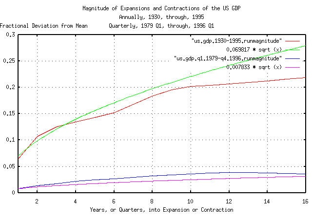
Figure VII is a plot of the annual and quarterly deviation from the
mean of the expansions and contractions of the US GDP, with the
theoretical values of 0.069817 * sqrt
(t) for the annual and 0.007833 * sqrt
(t) for the quarterly data. The astute reader would
note the discrepancy between the two values-they should be related by
a Brownian motion/random walk fractal scaling factor of
sqrt (4) = 2; the result of using
massaged data for analysis.
|
As a side bar, the dynamics of the USGDP are not,
necessarily, inconsistent with macro/micro economic
concepts. The root-mean-square and average of the USGDP's
marginal increments, However, manipulation of the variables through monetary or
fiscal policy to achieve a desired end may be problematical,
since the dynamics of the USGDP are dominated, at any one time,
by random processes. The deviation of the USGDP from its median
value, (which may be a Nash
equilibrium, but almost certainly not a Walrasian
general equilibrium,) can be quite significant for extended
periods of time as shown by Equation
(3.1) and Equation
(3.2), and illustrated in Figures VI and VII. The effects of
manipulation of the variables would be best confirmed by the
methodology used in the Instantaneous dynamic control of a GDP to regulate stochastic fluctuations is probably not attainable without excessive manipulation of the variables, which could, also, result in stability related issues. The problem is the magnitude of the stochastic dynamics represented by Equation (3.2) in relation to the effects that can be achieved through manipulation of the mechanisms of monetary and fiscal policy in the short term. |
The historical time series of the US GDP, from 1947Q1 through 2002Q1, inclusive, was obtained from http://www.bea.doc.gov/bea/dn/nipaweb/DownSS2.asp, file Section1All_csv.csv, and Table 1.2. Real Gross Domestic Product Billions of chained (1996) dollars; seasonally adjusted at annual rates, manipulated in a text editor to produce the US GDP time series us.gdp.q1.1947-q1.2002.
Sampling the time series at intervals, i =
4, (the data is in calendar quarters,) and finding the
average, avg, and, root-mean-square,
rms, respectively, of the US GDP time
series' marginal increments:
tssample -i 4 us.gdp.q1.1947-q1.2002 | tsfraction | tsavg -p
0.034609
tssample -i 4 us.gdp.q1.1947-q1.2002 | tsfraction | tsrms -p
0.043977
The probability of an annual up movement,
P, from Section
I, in the US GDP is:
avg
--- + 1
rms
P = ------- ........................................(1.24)
2
or P = 0.89348977875, and the
exponential marginal gain per unit time,
g, is:
P (1 - P)
g = (1 + rms) (1 - rms) ....................(1.20)
or g = 1.03423643697.
Note that the root-mean-square, rms,
of the marginal increments of the US GDP is a metric of risk; it
represents the probability, (more correctly, the frequency
distribution,) of catastrophes, large and small. From the
root-mean-square, the probability of catastrophes, over time, can be
calculated.
From Figure I, above:
(1.03423643697^t) * e^(-0.043977 * sqrt (t)) =
K * (1.03423643697^t) ..........................(3.9)
or
-0.043977 * sqrt (t) = ln (K) ......................(3.10)
where K specifies how much an economy
can decline, compared with the recent past, before the economy
collapses, (and probably deteriorates into social anarchy.) We have
some idea of the value of K from the
economic upheavals of the 1990's during the Asian
Contagion, the financial crisis in the Latin American republics,
and the middle European nations, including Russia. It appears that
when K = 0.65, (meaning the economy
declined 35%,)the economy is no longer capable of supporting
itself.
Solving Equation (3.10):
-0.043977 * sqrt (t) = ln (0.65) = -0.430782916 ....(3.11)
Or t = 95.9545878733 years-about a
century-using the US GDP as representative numbers for an economy in
general.
What Equation (3.11) says is that for any given century, one standard deviation, (about 84%,) of the economies that started the century will survive to the end of the century.
Likewise, the probability that an economy would survive two
centuries is 0.84 * 0.84 = 0.71 = 71%,
and four centuries, 0.71 * 0.71 = 0.50 =
50%, or half of the economies in history would last
less than four centuries, and half more, which is in fair agreement
with the historical record.
The ancient Egyptian civilization lasted about 30 centuries-longer
than any other civilization in history. The probability of a
civilization/economy lasting 30 centuries is 0.84^30 =
0.00535 which is about one in 187, which is reasonably
consistent with the historical record, too.
|
As a side bar, note that economic catastrophes-of a magnitude sufficient to destabilize a civilization-can be endogenous or exogenous, and its both the magnitude and duration of the catastrophe that determines whether the civilization will be destabilized. Such catastrophes are a high entropy agenda-happening without rhyme or reason. In this case, a century was chosen as the time scale-to be
consistent with historians who do it that way, (its really
fractal, and the analysis holds true for all time scales, by
altering the value of For example, the Roman Empire did not make it through the fourth century; an economic catastrophe that lasted the entire century-it took a century of bad economic fortune to destabilize the millennia old Roman Empire. Likewise, for example, the South American Inca civilization lasted a little more than a century before an exogenous event of unprecedented magnitude, (the invasion of the Spanish Conquistadors,) quickly toppled the empire-in less than a decade. What Equation (3.10) says is that there is a limit, (with a
metric As a simple interpretation of Equation (3.10), is that half of the economies in history lasted less than four centuries, and half more. |
Note that, although the duration of a GDP/civilization can never be
forever, it can be optimally maximized. Basically, it means maximizing
the growth of the GDP/civilization by manipulating both the
root-mean-square, rms, and average,
avg, of the GDP's marginal increments,
(perhaps though policy mandates.) See Equation Equation
(1.18) in the Optimization
section of Section
I of this series for particulars, (which may be inconsistent with
the tactical political expediencies of a policy of full employment,
etc.)
It is probably the case that similar limitations exist on the
durability and longevity of civilization itself, (and/or the global
GDP,) as a whole-which is a good reason for politicians to be
meticulously careful with the decision of waging war; destruction in
war affects both the root-mean-square,
rms, and average,
avg, of the marginal increments of the
global GDP, (and/or civilization,) in negative ways, (the
rms gets larger, and the
avg gets smaller,) escalating the risk
of global catastrophe. (Note that a war with no destruction only
increases the value of rms-the metric of
risk-since the outcome of any war is uncertain; a war with no
destruction is a zero-sum game-what one side wins, the other
loses. But it still increases the risk of catastrophe, to both sides,
and the global aggregate by increasing the value of
rms.)
Note that this analysis uses non-linear high entropy methodology, (specifically, log-normal system evolution,) to analyze the duration of economies and/or civilizations, and does not address the finer issues of leptokurtosis in frequency distributions of the margins, or non-linear dynamical system, (e.g., chaotic,) characteristics-which is the prevailing wisdom of most political economists. It does, however, give a representative distribution for the durations of civilizations that agree with the historical record.
The file
ic-na.q1.1979-q4.1996 contains
the time series history of the quarterly North American semiconductor
IC revenue, from Q1, 1979, through, Q4, 1996, (72 quarters,)
inclusive. The data is from the US DOC, file QSUSICXX, and references
Semiconductor Industry Association, (SIA,) running average data.
The data set is pitifully small, and the annual running average is not an appropriate choice for analyzing the dynamic characteristics of a time series.
Analysis:
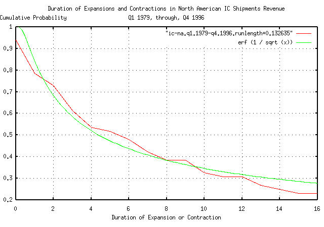
The cumulative probability of the duration between the North American IC revenue's values crossing its median value:
tsmath -l ic-na.q1.1979-q4.1996 | tslsq -o | \
tsrunlength > ic-na.q1.1979-q4.1996.runlength
wc ic-na.q1.1979-q4.1996
72 72 645 ic-na.q1.1979-q4.1996
tsshannoneffective -e dummy dummy 72
erf (1 / sqrt (72)) = 0.132635, 1 - erf (1 / sqrt (72)) = 0.867365
tsmath -l ic-na.q1.1979-q4.1996 | tslsq -o | tsrunlength | \
cut -f1,7 | tsmath -a 0.132635 > 'ic-na.q1.1979-q4.1996.runlength+0.132635'
where the entire cumulative distribution was missing past 72
quarters-the theoretical distribution past this value, from the
tsshannoneffective
program, was added to the emperically derived distribution.
|
Figure VIII is a plot of the cumulative probability of the duration
of the quarterly expansions and contractions of the North American IC
revenue with the theoretical value, erf (1 / sqrt
(t)).
The deviation from the mean of the expansions and contractions of the North American IC revenue:
tsmath -l ic-na.q1.1979-q4.1996 | tslsq -o | \
tsrunmagnitude > ic-na.q1.1979-q4.1996.runmagnitude
tsfraction ic-na.q1.1979-q4.1996 | tsrms -p
0.083072
|
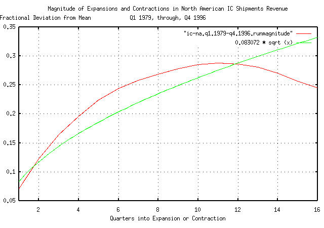
Figure IX is a plot of the quarterly deviation from the mean of the
expansions and contractions of the North American IC revenue, with the
theoretical value of 0.083072 * sqrt
(t). The tsrunmagnitude
program is sensitive to both data set size and massaging of
data which accounts for the extreme drop off in the empirical analysis
past 12 quarters.
|
As a side bar, Equation (1.18) is a very useful and important equation. For example: meaning that from Equation (1.24): But from Equation (1.18): An interpretation of this result is that the optimal risk for
a company in the North American IC market is to place about 50%
of the company's value at risk, every quarter, and the maximum
sustainable debt to equity ratio, (or capitalization to equity
ratio, depending on how one wants to interpret it,) is
for a maximum sustainable growth rate of about 14% per
quarter, which is about 70% per year, or maximum sustainable
growth rate of just under a factor of two per year, albeit with
fairly significant capitalization, (but the optimal solution
would be for 100% ROI-in shareholder equity, if that's they way
one wants to interpret it-in 3.43 years, too!) Note that it is
an optimal solution-infusing less, or more,
capital than optimal would yield inferior results. Additionally,
if one wants to interpret it as a valuation, a company that is
running optimal will have a valuation of about
Interestingly, many of the better companies in the North American IC marketplace between 1979 and 1995 sustained annual growth rates near a factor of two, (most of them smaller companies where an annual growth rate of two could be managed.) During that time, a factor of three times the gross revenue of a company was used by the investment banking and venture capital industry as a benchmark valuation factor. |
The file
ge.jan.02.1962-feb.15.2002
contains the time series of GE's daily close equity price history,
from January 2, 1962, through, February 15, 2002, (10,103 days,)
inclusive. The data is from the Yahoo!'s Historical Prices database, and
is adjusted for splits.
The file was converted to a Unix flat file database with the
csv2tsinvest
program:
csv2tsinvest GE ge.csv > ge.jan.02.1962-feb.15.2002
Analysis:
The cumulative probability of the duration between GE's equity price value crossing its median value:
tsmath -l ge.jan.02.1962-feb.15.2002 | tslsq -o | \
tsrunlength | cut -f1,7 > ge.jan.02.1962-feb.15.2002.runlength
|
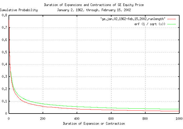
Figure X is a plot of the cumulative probability of the duration of
the expansions and contractions in GE's equity price with the
theoretical value, erf (1 / sqrt
(t)).
The deviation from the mean of the expansions and contractions of in GE's equity price:
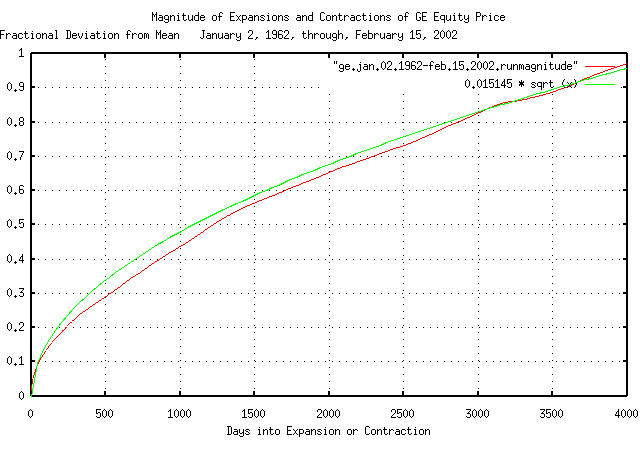
tsfraction ge.jan.02.1962-feb.15.2002 | tsrms -p
0.015145
tsmath -l ge.jan.02.1962-feb.15.2002 | tslsq -o | \
tsrunmagnitude > ge.jan.02.1962-feb.15.2002.runmagnitude
|
Figure XI is a plot of the deviation from the mean of the
expansions and contractions of GE's equity price, with the theoretical
value of 0.015145 * sqrt (t).
|
As a side bar for intuitive development, Figure X and Figure XI look the way they do because a shareholder's predictions or expectations are self-referential and deductively indeterminate. For example, suppose an equity's value decreases. Some would decrease their position in the equity to avoid further losses-others would see it as a buying opportunity. Both hypothesis are subjective and equally defensible. J. M. Keys (General Theory of Employment, Interest and Money, London, Macmillan, 1936,) summed up self-referential indeterminacy in the equity market as: [a market strategy means determining] what the average opinion expects the average opinion to be. As the agents in a market struggle with the self-referential indeterminacy, (which, incidentally, pervades all of economics,) their actions will have random characteristics, (i.e., some will buy on a certain kind of market information, others will sell on the same information.) This indeterminacy is the random mechanism in equity prices. Now, as a simple market concept, suppose those intending to buy or sell an equity line up in a queue-a waiting line to make their transactions. Each person can see what the previous transaction price of the equity was by observing the transaction of the person in front of them-a simple equity market ticker model. To sell shares, the selling price has to be lowered below the existing price, i.e., the price set by the previous person in the queue-and, likewise, to buy shares, the price has to be raised. For simplicity, suppose that to sell, the price is lowered by 1%, and to buy, raised by 1%-a simple arbitrage model. So, what we have, through a day of trading, is a series of transactions that, randomly, (depending on the subjective trading hypothesis of the individual investors,) either move the price of an equity up by 1%, or down by 1%, from the equity's immediate preceding price. The value of the equity at the end of the trading day would be determined by the last transaction, which would be the result of a geometric progression of moving the equity's price either positive by 1%, or negative by 1%, through the day, in a random fashion, (the Brownian motion/random walk fractal equivalent, described in Section II, of the trading day would be a fixed increment fractal with a binomial distribution.) Over many trading days, the Brownian motion/random walk
fractal equivalent's distribution of the marginal increments of
the closing value of the equity would approach a Gaussian/normal
distribution, (for an example, see GE's equity price, Figure
II from Section
I.) In point of fact, that is exactly how the
And, that is a simplified explanation why Figure X and Figure XI look the way they do. The dynamics are characteristic-with all their bubbles, crashes, etc.-of any non-linear high entropy economic system. The study of why aggregate systems behave this way is called complexity theory, and game theory is the study of self-referential indeterminacy and its relation to conflict of interest. As an interesting historical note, the concept of relating game-theoretic characteristics of iterated games-as a causality- to their effect on the fractal dynamics of an economic system as an optimization abstraction is not new; for example, it was proposed by in Games and Decisions: Introduction and Critical Survey, R. Duncan Luce and Howard Raiffa, Dover Publications, Inc., New York, New York, 1957, ISBN 0-486-65943-7, pp. 483, almost a half-century ago. |
It is not clear whether the characteristics of project completion exhibit non-linear high entropy or Brownian Motion/random walk dynamics. However, since most projects are of relatively short duration, the difference between the characteristics of the two is small, and either can be used.
If project milestone completion, c,
is considered a linear function of resource allocation, (i.e.,
c = kt,) and the project's decision
process has sufficiently high entropy, then the real milestone
completion for projects would have a distribution that has a deviation
closer to c = sqrt (kt).
In other words, the ratio of the projected milestone completion, to
the measured would be sqrt (kt); the
typical project would have less than sqrt
(kt) milestone's finished, for one deviation of the
time, (i.e., 84.1% of the projects would be less than
sqrt (kt) finished-where they should be
kt finished-and 15.9% would be greater
than sqrt (kt) finished.)
Or, 1 / 0.841 = 1.19 deviations of
all projects would be better than on schedule and on budget, which is
11.7%; and the remaining 88.3% would not.
Its interesting because it is less than a 5% error with the industry metrics maintained by Standish Group's, Jim Johnson, which authored http://www.standishgroup.com/sample_research/chaos_1994_1.php, http://www.scs.carleton.ca/~beau/PM/Standish-Report.html, and, http://www.garynorth.com/y2k/detail_.cfm/1088.
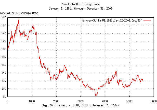
The historical time series of the Yen/DollarUS' 5549 daily closes,
from January 2, 1981 through December 31, 2002, inclusive, was
obtained from PACIFIC -
Policy Analysis Computing & Information Facility In Commerce's
historical currency database, PACIFIC - FX
Retrieval Interface, and the format manipulated with a text
editor-filename
Yen-per-DollarUS.1981.Jan.02-2002.Dec.31.
|
Figure XII is a plot of the daily closes of the Yen/DollarUS exchange rate, from January 2, 1981 through December 31, 2002. The maximum exchange rate was 277.66 on November 4, 1982, (day 463,) and the minumum, 81.071, on April 19, 1995, (day 3612).
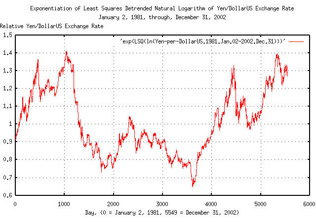
Converting the daily closes of the Yen/DollarUS exchange rate to its Brownian motion/random walk equivalent time series, de-trending, and re-exponentiating, as suggested in Section II:
tsmath -l Yen-per-DollarUS.1981.Jan.02-2002.Dec.31 | \
tslsq -o | tsmath -e > 'exp(LSQ(ln(Yen-per-DollarUS.1981.Jan.02-2002.Dec.31)))'
|
Figure XIII is a plot of the de-trended daily closes of the Yen/DollarUS exchange rate, from January 2, 1981 through December 31, 2002. On day 1038, (note the shift from day 463, where the exchange rate was a factor of 1.36506 times its median value,) the Yen/DollarUS exchange rate was 1.410831 times its median value, and on day 3612, it was a factor of 0.645174; or in the 22 year interval, the maximum divided by the minimum was a little less than a factor of 2.2.
tsmath -l Yen-per-DollarUS.1981.Jan.02-2002.Dec.31 | tslsq -o | tsderivative | \
tsnormal -t > Yen-per-DollarUS.1981.Jan.02-2002.Dec.3.std.distribution
tsmath -l Yen-per-DollarUS.1981.Jan.02-2002.Dec.31 | tslsq -o | tsderivative | \
tsnormal -t -f > Yen-per-DollarUS.1981.Jan.02-2002.Dec.3.distribution
|
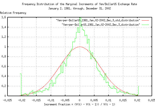
Figure XIV is a plot of the frequency distribution of the marginal increments of the Brownian motion/random walk equivalent of the daily closes of the Yen/DollarUS exchange rate, from January 2, 1981 through December 31, 2002. Note the leptokurtotsis.
|
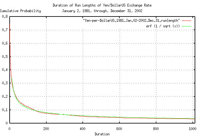
Figure XV is a plot of the cumulative probability of the duration
of the expansions and contractions of the Brownian motion/random walk
equivalent of the Yen/DollarUS exchange rate, from January 2, 1981
through December 31, 2002 with the theoretical value,
erf (1 / sqrt
(t))
. The frequency of
durations of up to 1012 business days, (about 4 calendar years,) are
shown.
    tsfraction Yen-per-DollarUS.1981.Jan.02-2002.Dec.31 | tsrms -p
    0.006886
|
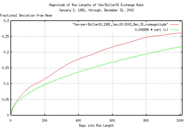
Figure XVI is a plot of the deviation from the mean of the
expansions and contractions of the Brownian motion/random walk
equivalent of the Yen/DollarUS exchange rate, from January 2, 1981
through December 31, 2002, with the theoretical value of
0.006886 * sqrt (t). The deviation of
expansions, or contractions, of up to 1,012 business days, (about 4
calendar years,) are shown.
For example, the effect that Yen/DollarUS fluctuations would have
on an international manufacturer that manufactured products in one one
country, and sold them in another-assuming the transportation;
distribution; retail chain cycle, etc., was 20, (about a calendar
month,) business days-would be e^(0.006886 * sqrt (20))
= 1.03127420323, or about 3%. Or, one standard
deviation of the time, about 84% of the time, the manufacturer would
get a windfall of 3%, and 84% of the time, a shortfall of 3%.
Fluctuations in international currency exchange rates can have significant financial implications for vendors in retail markets, where margins run a few percent-a company can show negative cash flow for a significant fraction of a calendar year depending on the lottery of the international currency markets.
|
As a side bar, almost all international trade is hedged against currency fluctuations. As a simple example, if an international manufacturer and a local retailer agree to exchange money-at a future date-in exchange for products at a specified price, then both are protected against the negative implications of currency fluctuations; but they don't get advantages of a favorable fluctuation, either. The agreement is called paper, and it is a derivative, and since risk is transfered, it is called a hedge. Usually, the paper is administered through a derivative trader, (commonly, an international bank,) and has value-it can be sold, or bought. The OTC derivatives markets are the largest, dollar-wise, markets in the world, from "Financial Engineering News", June/July, 2002, Issue No. 26, pp. 3:
Just as a perspective, the World's currency markets do about $1.4 trillion a day-about what the entirety of the US equity markets do in a calendar quarter. Money itself is big business. |
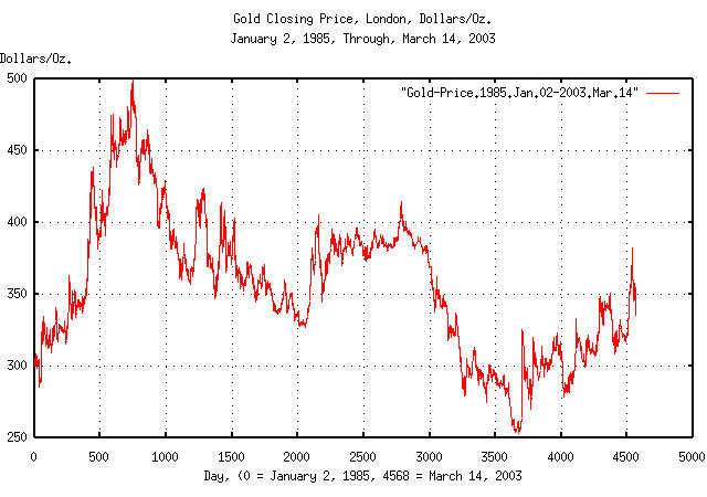
Gold price dynamics are often analyzed assuming the price has Brownian motion/random walk fractal characteristics. Although probably sufficiently accurate for short term analysis, there are logical contradictions extrapolating the paradigm to long term analysis; for example, there is nothing constraining gold prices to be non-negative. However, assuming gold price fluctuations to be a non-linear high entropy geometric progression with log-log distributed marginal increments resolves the problem.
The historical time series of the London gold price closes for 4568
daily closes, from January 2, 1985 through March 1, 2003, inclusive,
was obtained from The London Bullion
Market Association's London Market
Statistics, and the format manipulated with a text editor-filename
Gold-Price.1985.Jan.02-2003.Mar.14.
|
Figure XVII is a plot of gold's daily closing price, from January 2, 1985 through March 1, 2003. The maximum price was 499.75 on December 14, 1987, (day 745,) and the minumum, 252.80, on August 20, 1999, (day 3653).
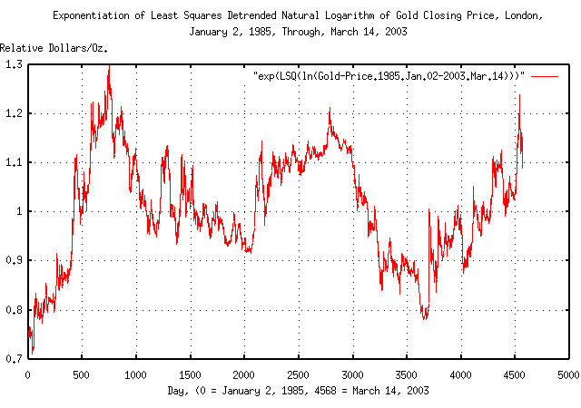
Converting gold's daily closing price to its Brownian motion/random walk equivalent time series, de-trending, and re-exponentiating, as suggested in Section II:
    tsmath -l Gold-Price.1985.Jan.02-2003.Mar.14 | \
        tslsq -o | tsmath -e > 'exp(LSQ(ln(Gold-Price.1985.Jan.02-2003.Mar.14)))'
|
Figure XVIII is a plot of the de-trended gold closing price, from January 2, 1985 through March 1, 2003. On day 745, gold's closing price was 1.297522 times its median value, and on day 39, it was a factor of 0.708065; or in the 18 year 2 month interval, the maximum divided by the minimum was a little less than a factor of 1.8. Note the shift in the minimum from day 3653 to day 39.
    tsmath -l Gold-Price.1985.Jan.02-2003.Mar.14 | tslsq -o | tsderivative | \
        tsnormal -t > Gold-Price.1985.Jan.02-2003.Mar.1.std.distribution
    tsmath -l Gold-Price.1985.Jan.02-2003.Mar.14 | tslsq -o | tsderivative | \
        tsnormal -t -f > Gold-Price.1985.Jan.02-2003.Mar.1.distribution
|
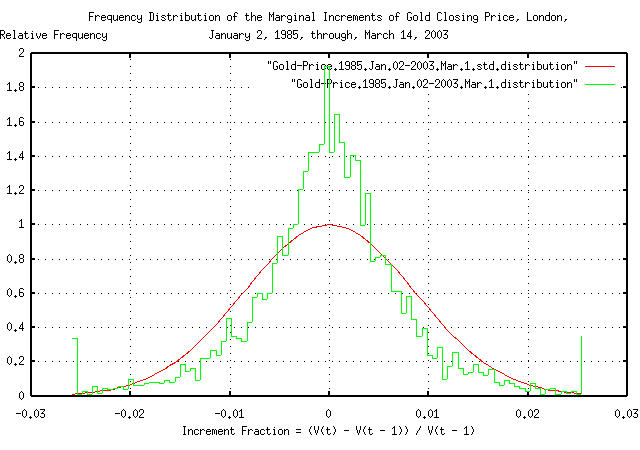
Figure XVIX is a plot of the frequency distribution of the marginal increments of the Brownian motion/random walk equivalent of gold's daily closing price, from January 2, 1985 through March 1, 2003. Note the leptokurtotsis.
|
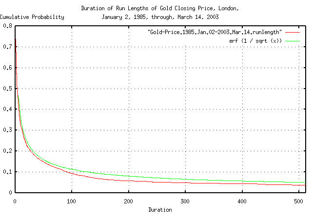
Figure XX is a plot of the cumulative probability of the duration
of the expansions and contractions of the Brownian motion/random walk
equivalent of gold's daily closing price, from January 2, 1985 through
March 1, 2003, with the theoretical value, erf (1 / sqrt
(t)). The frequency of durations of up to 506 business
days, (about 2 calendar years,) are shown.
    tsfraction Gold-Price.1985.Jan.02-2003.Mar.14 | tsrms -p
    0.008637
|
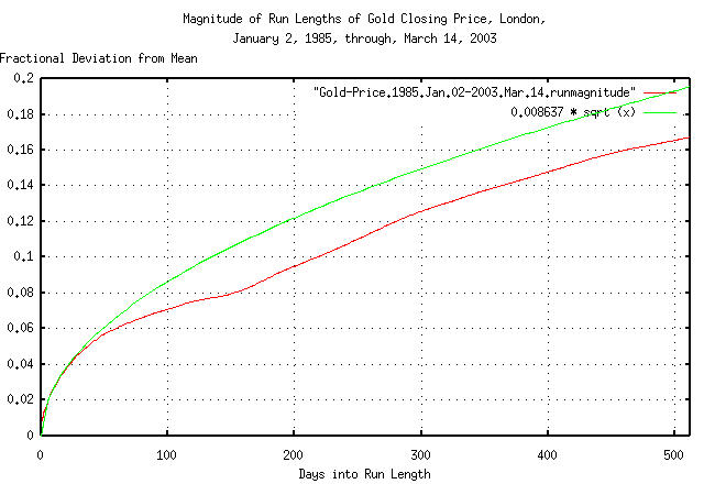
Figure XXI is a plot of the deviation from the mean of the
expansions and contractions of the Brownian motion/random walk
equivalent of gold's daily closing price, from January 2, 1985 through
March 1, 2003, with the theoretical value of 0.008637 *
sqrt (t). The deviation of expansions, or
contractions, of up to 506 business days, (about 2 calendar years,)
are shown.
    tsmath -l Gold-Price.1985.Jan.02-2003.Mar.14 | \
        tslsq -o | tsroot -l > Gold-Price.1985.Jan.02-2003.Mar.14.root
|
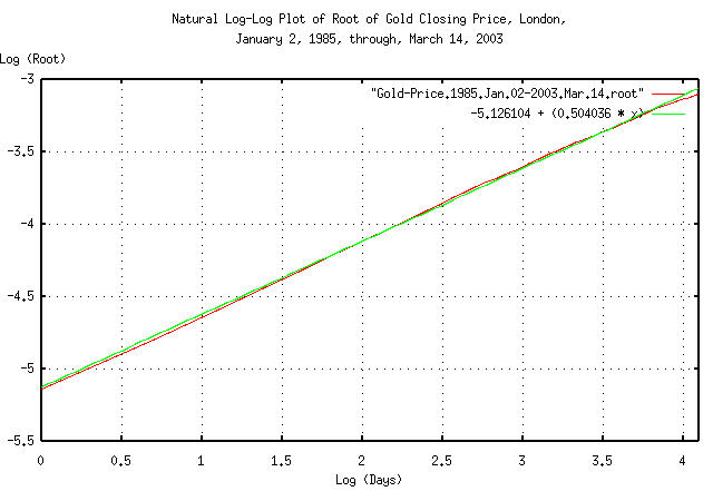
Figure XXII is a plot of the root, and the least-squares-best-fit,
of the expansions and contractions of the Brownian motion/random walk
equivalent of gold's daily closing price, from January 2, 1985 through
March 1, 2003, for e^4.09434456222 = 60
days, (about 3 calendar months.) The marginal increments do seem to
add root-mean-square, (0.5 v.s. 0.504036; the slope of the line is the
root.)
The historical time series of the CPIAI from January, 1913 through
May, 2003, inclusive, was obtained from the US Department of Labor, Bureau
of Labor and Statistics, Consumer
Price Index, All Urban Consumers - (CPI-U), and edited in a text
editor to make a monthly time series, filename cpiai.1913.Jan-2003.May.
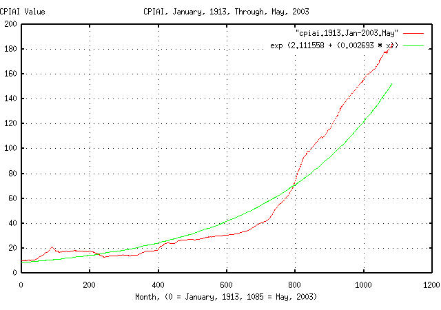
Note that the time series is US inflation/deflation monthly rates, based on a basket of goods, and not asset valuations, (although about 41% of the recent weights was housing and shelter; see Table 1 (1993-95 Weights), Relative importance of components in the Consumer Price Indexes: U.S. city average, December 2001, for particulars.) The asset value time series is available, (see Fixed Asset Tables,) but only include data since 1996. Additionally, the inflation/deflation time series is produced using a geometric filtering technique, as explained at Note on a New, Supplemental Index of Consumer Price Change, which is why Figure XXIII appears to be too smooth.
    tslsq -e -p cpiai.1913.Jan-2003.May
    e^(2.111558 + 0.002693t) = 1.002696^(784.223106 + t) = 2^(3.046334 + 0.003885t)
|
Figure XXIII is a plot of the monthly CPIAI values, from January,
1913 through May, 2003, and the least-squares exponential best fit
from the tslsq
program. The inflation over the period averaged 0.2696% per month,
which is an annual rate, (1.0002696^12 =
1.03283605276,) of about 3.3% per year.
Converting the CPIAI time series to its Brownian motion/random walk equivalent time series, de-trending, and re-exponentiating, as suggested in Section II:
    tsmath -l cpiai.1913.Jan-2003.May | \
        tslsq -o | tsmath -e > 'exp(LSQ(ln(cpiai.1913.Jan-2003.May)))'
|
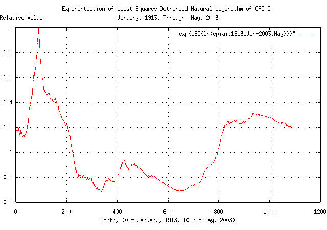
Figure XXIV is a plot of the CPIAI's de-trended, re-exponentiated, Brownian motion/random walk equivalent time series from January, 1913 through May, 2003.
|
As a side bar, the interesting events, (see, also, Example I, the DJIA, above,) in Figure XXIV:
Its rather obvious that the stock market crash of 1929 didn't create the Great Depression-it was a result of it. The stock market crash was was a part of a larger, more general, asset deflation that started in the early 1920's. (There is some speculation, if inflation is representative of asset values-that capital moved out of assets-which were decreasing through the early 1920's-and into the equity markets, making an equity market bubble, which crashed in 1929; but know one really knows for sure.) Note that the deflation in the Great Depression was not
insignificant. |
    tsmath -l cpiai.1913.Jan-2003.May | tslsq -o | \
        tsrunlength | cut -f1,7 > cpiai.1913.Jan-2003.May.runlength
|
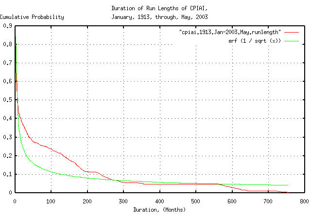
Figure XXV is a plot of the cumulative probability of the duration of periods of inflation and deflation of the Brownian motion/random walk equivalent of the CPIAI, from January, 1913 through May, 2003. Note that since the US Department of Labor, Bureau of Labor and Statistics uses a geometric filtering technique, as described in Note on a New, Supplemental Index of Consumer Price Change, the relative number of short term durations is too small, pushing up the relative number of mid-term durations in the distribution.
tsfraction cpiai.1913.Jan-2003.May | tsrms -p
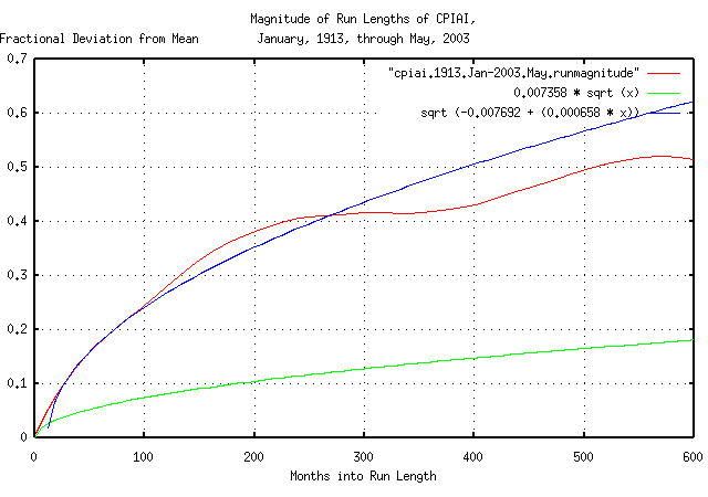
0.007358
tsmath -l cpiai.1913.Jan-2003.May | tslsq -o | \
tsrunmagnitude > cpiai.1913.Jan-2003.May.runmagnitude
head -100 cpiai.1913.Jan-2003.May | tail -88 | tslsq -R -p
sqrt (-0.007692 + 0.000658t)
|
Figure XXVI is a plot of the deviation from the mean of the
expansions and contractions of the Brownian motion/random walk
equivalent of the CPIAI, from January, 1913 through May, 2003. Note
that since the US Department
of Labor, Bureau of Labor and Statistics uses a geometric
filtering technique, as described in Note on a New, Supplemental
Index of Consumer Price Change, the short term deviation is too
small. However, an approximation to the monthly deviation of the
inflation/deflation can be extrapolated by measuring the deviation
between months 12 and 100, (i.e., for 88 months,) which gives a
monthly deviation value, rms = sqrt (0.000658) =
0.0256515107.
|
As a side bar, what are the chances of an inflation/deflation period happening that is similar to the Great Depression? We have to look at the duration, and the depth. The deflation of the Great Depression started in September,
1931, and ended in April, 1979, for a total duration of 571
months. The chances of a similar period of deflation lasting at
least 571 months is The deflationary crash started in June, 1920, and
bottomed in May, 1933, (a total of 155 months,) during which
prices, (or approximately asset values,) decreased by a factor
of |
As a useful approximation to Equation
(3.7), where t is small, after
exponentiating both sides:
                     -N * (rms * sqrt (t))
    Vo / Vi = g^t * e                      .............(3.12)
But for Vo / Vi near unity,
ln (Vo / Vi) is approximately
Vi - 1, and
g^t is approximately unity for
t small, or:
Vo - 1 = -N * rms * sqrt (t) .......................(3.13)
and using the approximation for Equation (3.7):
0.1 - 1 = 0.9 = -N * 0.01 * sqrt (400) .............(3.14)
or N = 4.5 deviations, which
corresponds to a conservative estimate of a
0.000003397672912712 chance, which is a
frequency rate of approximately 294,319
trading days, on average, which is 1,163
years of 253 trading days per year. Call it a
once-a-millennia-event.
Why does the approximation work?
For small values of time, t, the
characteristics of the non-linear high entropy system are almost the
same as its Brownian motion/random walk equivalent without the
exponential transformations-the log-normal characteristics evolve over
time from the normal/Gaussian characteristics. As an approximation,
for t small, the exponentiation, and the
inverse operations are almost unity, i.e., ln (1 +
t) is about t, and
e^t is about 1 +
t for t small.
The error function, erf (), operator
is approximately unity for t >> 1
meaning that erf(1 / sqrt (t)) is
approximately 1 / sqrt (t) for
t large.
--

John Conover, john@email.johncon.com, http://www.johncon.com/