Quantitative Analysis of Non-Linear High Entropy Economic Systems I

From: John Conover <john@email.johncon.com>
Subject: Quantitative Analysis of Non-Linear High Entropy Economic Systems I
Date: 14 Feb 2002 07:38:46 -0000

Introduction

Much of applied economics has to address non-linear high entropy systems-those systems characterized by random fluctuations over time-such as equity prices, gross domestic product, industrial markets, etc.

An optimal wagering strategy for high entropy systems was first suggested by Claude Shannon in the mid 1940's in his pioneering work on information theory, The Mathematical Theory of Communication, (pp. 39-42.) The concept was further refined by J. L. Kelly Jr. in the Bell System Tech. J. vol. 35, 1956, A New Interpretation of Information Rate, (pp. 917-926), which established the isomorphism between the information-theoretic concept of information rate in a binary symmetric channel and speculation under uncertainty. More recently, Fazlollah M. Reza in An Introduction To Information Theory, (pp. 450-452,) has offered an alternative derivation that requires only the concepts of the law of large numbers, and the maxima from calculus-both taught in freshman mathematics-to derive the same optimal wagering strategy.

Note: the C source code to all programs used are available from the NtropiX Utilities page, or, the NdustriX Utilities page, and are distributed under License.

Optimization

Following Reza, suppose a gambler wagers on an iterated game of chance. Further, suppose there is a chance, P, of the gambler winning any iteration of the game, and of 1 - P, of losing. Let the capital the gambler starts with be V(0), and V(t) the capital after the t'th iteration of the game. Since the gambler is not certain of the outcome of any iteration of the game, only a fraction, f, of the capital is wagered on each iteration of the game. Thus, after t many iterations the capital is:

                  w          l
    V(t) = (1 + f)  * (1 - f)  * V(0) ..................(1.1)

where w is the number of times the gambler won, and l = t - w, the number of times the gambler lost. These numbers are functions of two random variables, denoted by W and L. Then, by the law of large numbers:

                   1
    lim            - W = P .............................(1.2)
       t->infinity t

and:

                   1
    lim            - L = q = 1 - P .....................(1.3)
       t->infinity t

The gambler must determine the fraction, f, of the capital to wager on each iteration of the game, which will maximize the average exponential growth rate, G, of the capital, i.e., maximize the value of:

                       1     V(t)
    G = lim            - ln (----) .....................(1.4)
           t->infinity t     V(0)

with respect to f:

                       W              L
    G = lim            - ln (1 + f) + - ln (1 - f) .....(1.5)
           t->infinity t              t

or:

    G = P ln (1 + f) + q ln (1 - f) ....................(1.6)

which, by taking the derivative with respect to f, and equating to zero, is maximal when:

    dG            P - 1        1 - P
    -- = P (1 + f)      (1 - f)
    df

                 1 - P - 1        P
        - (1 - P)          (1 + f)  = 0 ................(1.7)

and, combining terms:

             P - 1        1 - P
    P (1 + f)      (1 - f)

                         P        P
        - (1 - P) (1 - f)  (1 + f)  = 0 ................(1.8)

and, splitting:

             P - 1         1 - P
    P (1 + f)      (1 - f)

                         P        P
        = (1 - P) (1 - f)  (1 + f)  ....................(1.9)

Taking the logarithm of both sides:

    ln (P) + (P - 1) ln (1 + f) + (1 - P) ln (1 - f)

        = ln (1 - P) - P ln (1 - f) + P ln (1 + f) .....(1.10)

and combining terms:

    (P - 1) ln (1 + f) - P (ln (1 + f) + (1 - P) ln (1 - f)

        + P ln (1 - f) = ln (1 - P) - ln (P) ...........(1.11)

or:

    ln (1 - f) - ln (1 + f) = ln (1 - P) - ln (P) ......(1.12)

and performing the logarithmic operations:

        1 - f        1 - P
    ln (-----) = ln (-----) ............................(1.13)
        1 + f          P

and exponentiating:

    1 - f   1 - P
    ----- = ----- ......................................(1.14)
    1 + f     P

reduces to:

    P (1 - f) = (1 - P)(1 + f) .........................(1.15)

and expanding:

    P - P f = 1 - P f - P + f ..........................(1.16)

or:

    P = 1 - P + f ......................................(1.17)

and, finally:

    f = 2 P - 1 ........................................(1.18)

Substituting, q, from Equation (1.3) into Equation (1.6):

    G = P ln (1 + f) + (1 - P) ln (1 - f) ..............(1.19)

where G is the average exponential growth rate of the gambler's capital, per iteration of the game. As a useful form, exponentiating both sides:

               P        (1 - P)    G
    g = (1 + f)  (1 - f)        = e  ...................(1.20)

where the gain, g, is the average multiplicative gain per iteration of the game, i.e., after t many iterations, the gambler's capital would have increased by a factor of g^t.

    srms = sqrt (rms^2 - avg^2)
    G = avg - (srms^2 / 2)
    g = e^(avg - (srms^2 / 2))

Equation (1.18) and Equation (1.20) are important. As a simple example, suppose each outcome of an iterated game depends on a throw of a fair six sided die-if the die comes up four, or less, the gambler wins what was wagered; else loses it. The gambler's optimal strategy is to put 1 / 3 of the capital at risk, (by wagering it,) on each iteration of the game, since P = 4 / 6, and from Equation (1.18), f = 2 P - 1 = 1 / 3. The gambler's capital would increase, from Equation (1.20), on average, by a factor of g = 1.05826736798 per iteration of the game, or about 6% per game.

But how does the gambler play the game if the value for P is unknown?

Equation (1.20) offers a metric methodology. For the t'th iteration of the game, the fractional gain, f(t), in the gambler's capital for the iteration is:

           V(t) - V(t - 1)
    f(t) = --------------- .............................(1.21)
              V(t - 1)

The absolute value of f(t) is the fraction of the capital the gambler wagered on the t'th iteration of the game-it is the fraction of capital that the gambler put at risk, f. The capital increased if the gambler won on the game in the t'th iteration, and decreased if the gambler lost-by the fraction of the capital the gambler put at risk, f.

If n has a sufficiently large data set size, then by the law of large numbers, in n many iterations of the game, the total number of wins for the gambler would be expected to be n P and the total number of losses would be expected to be n (1 - P), for an average number of wins of (n P - n (1 - P)) / n = 2 P - 1. The average gain, avg would then be:

    avg = (2 P - 1) f ..................................(1.22)

where f is the return on the fraction of capital wagered on each iteration of the game, (srms,) and is equal to rms, the root-mean-square of the marginal increments of the capital, and avg is the mean of the marginal increments of the capital. Solving for P:

    avg
    --- = 2 P - 1 ......................................(1.23)
    rms

or:

        avg
        --- + 1
        rms
    P = ------- ........................................(1.24)
           2

The interpretation of P is that it is the likelihood of up movement in the characteristics of a high entropy economic system.

Substituting Equation (1.18) for P in Equation (1.24), and letting f = rms:

               avg
               ---- + 1
    rms + 1    rms
    ------- =  -------- ................................(1.25)
       2          2

or, maximal growth occurs when:

             2
    avg = rms  .........................................(1.26)

          V(t) = V(t - 1) * (1 + a(t)) .....................(1.27)

      

           V(t) = V(t - 1) * (a + b * V(t - 1)) =

                                  2
                  a V(t - 1) + b V (t - 1) .................(1.28)

      

The concept is similar to automating risk arbitrage, based on historical performance, where an expected-value table of the difference between an investment's potential upside, (multiplied by the probability of achieving the potential upside,) and the the potential downside, (multiplied by the probability of the downside occurring,) is the expected value of the return of the investment-the difference between the potential upside and potential downside corresponding to the root-mean-square, rms, of the value of the investment, and the average, avg, the expected value, where P is the likelihood of the potential upside occurring.

Important Formulas

Reiterating the important equations for high entropy economic systems:

        avg
        --- + 1
        rms
    P = ------- ........................................(1.24)
           2

                 P          (1 - P)
    g = (1 + rms)  (1 - rms)        ....................(1.20)

and for maximal growth:

    rms = 2 P - 1 ......................................(1.18)

which is when:

             2
    avg = rms  .........................................(1.26)

where avg is the mean, and rms the root-mean-squre, of the system's marginal increments.

Of interest is that only two variables,avg and rms, are involved in optimizing the performance of a high entropy economic system. Typical values for avg and rms are 0.0004 and 0.02, respectively, for daily data. P would then have a value of 0.51, and g a value of 1.0002 per day, which is about 5% per calendar year, for 253 business days in a calendar year.

Example I, GE Equity Price

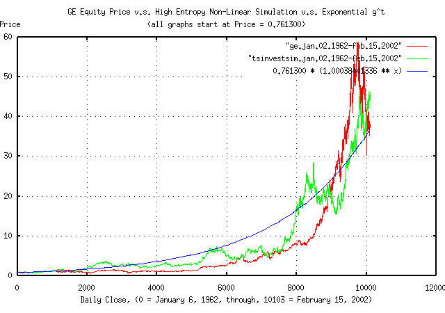
As an emperical exercise to demonstrate the usage of Equation (1.24) and Equation (1.20), the equity price history for General Electric, (ticker symbol, GE,) for the last 10,103 days, (January 4, 1962, to February 15, 2002,) was downloaded from Yahoo!'s Historical Prices database, and the csv2tsinvest program used to convert the database to a time series. The mean of the marginal increments of the price, avg, and the root-mean-square of the price, rms, was found to be 0.000499, and 0.015145, respectively, using the tsfraction, tsavg, and, tsrms programs. On January 4, 1962, the initial value of the equity was $0.761300, adjusted for splits. On February 15, 2002, the value was $37.11.

From Equation (1.24):

        0.000499
        -------- + 1
        0.015145
    P = ------------ = 0.516474084 .....................(1.29)
             2

And, from Equation (1.20):

                      0.516474084
    g = (1 + 0.015145)            *

                      (1 - 0.516474084)
        (1 - 0.015145)

      = 1.00779357225 * 0.992648138

      = 1.00038441336 ..................................(1.30)

Figure I is a plot of the GE's equity price, from January 4, 1962, to February 15, 2002, and the equation 0.761300 * 1.00038441336^t. Additionally, the tsinvestsim program was used to generate a time series with the same characteristics, (P = 0.516474084, I = 0.761300, and f = 0.015145,) using a uniformly distributed random number generator, to produce a binomial frequency distribution with 10103 elements to simulate a normal/Gaussian distribution, which is overlayed, also.

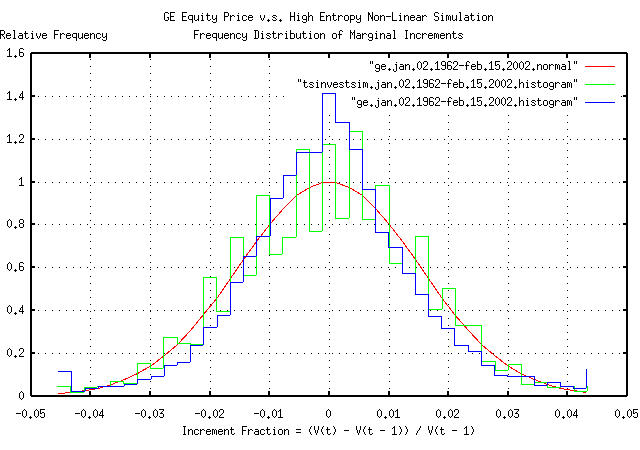
Figure II is the frequency distribution of the marginal increments of GE's equity price, from January 4, 1962, to February 15, 2002, and a least squares fit of the distribution to a Normal/Gaussian bell curve distribution. The binomial frequency distribution of the marginal increments of the time series simulated with the tsinvestsim program shown in Figure I is also displayed. The data in Figure II was made with the tsnormal program. The comb effect in the binomial frequency distribution was caused by aliasing between the binomial elements in the frequency distribution and the histogram element size of the plot, and could be removed by choosing a larger histogram element size. Of passing interest is the leptokurtosis in the frequency distribution of the marginal increments of GE's equity price, which is explored further in Example III.

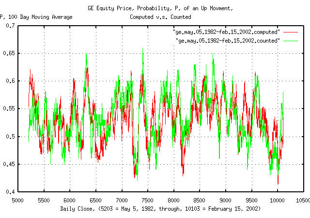
Figure III is a plot of the likelihood, P, of an up movement in GE's equity price as computed by the tsshannonwindow program for a 100 day moving window, from May 5, 1981 to February 15, 2002-4,900 business days for clarity. The first time series presents likelihood, P, computed by Equation (1.24) for the moving window. The second by counting the number of up movements in the window.

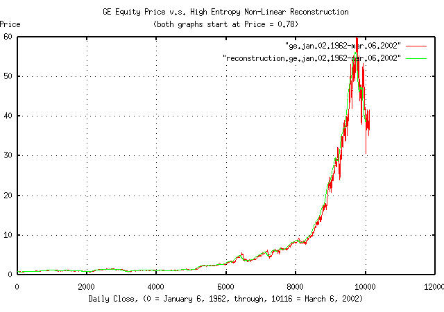
Figure IV is a plot of the reconstructed GE equity price time series, as computed by the tsgainwindow program for a 100 day moving window, from January 6, 1962 to March 6, 2002, overlayed on the original GE equity price. The tsgainwindow program uses Equation (1.24) and Equation (1.20) to derive the statistics of the time series for the moving window, which is then used for the reconstruction:

    tsgainwindow -w 100 ge.jan.02.1962-mar.06.2002 | tsmath -l | tsintegrate | \
        tsmath -e | tsmath -m 0.78 > reconstruction.ge.jan.02.1962-mar.06.2002

where "tsmath -l | tsintegrate | tsmath -e | tsmath -m 0.78" implements the geometric reconstruction by taking the natural logarithm of the series, integrating it, exponentiating it, and scaling it by a factor of 0.78, which was the initial value of the original time series.

Example II, Is the Equity Price Growth of the DJIA Component Companies Optimally Maximal?

If the component companies in the DJIA are the premier companies in the US exchanges, then their equity price characteristics should be near optimally maximal, i.e., consistent with Equation (1.26).

TABLE I contains the average, avg, the root-mean-square, rms, and the root-mean-square, squared, rms^2, of the marginal increments for the equity price time series for each of the component companies in the DJIA. The daily close equity price history for each component company in the DJIA was downloaded from Yahoo!'s Historical Prices database, and the csv2tsinvest program used to convert the database to a time series. The tsfraction, tsavg, and, tsrms programs were used to calculate the average, avg, and, the root-mean-square, rms, of the marginal increments of each time series. The tsmath program was used to square the rms values. The time series files represented from between January 2, 1962 and July 9, 1986 for the various component companies, to March 6, 2002.

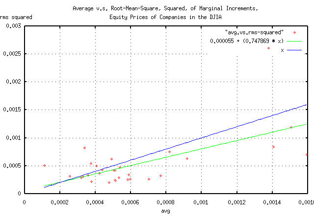
Figure V is a parametric scatter plot of the average v.s. the root-mean-square, squared, avg and rms^2, respectively, of the component companies of the DJIA. The figure is a pictographic representation of the data in TABLE I.

It does, indeed, appear that the equity price growth of most of the DJIA component companies is near optimally maximal, although slightly risk adverse.

Example III, Leptokurtosis In the Increments of the DJIA

The historical time series of the DJIA's 27949 daily closes, from January 2, 1900 through March 6, 2002, inclusive, was obtained from Yahoo!'s database of equity Historical Prices, (ticker symbol ^DJI,) in csv format. The csv format was converted to a Unix database format using the csv2tsinvest program, filename djia1900-2002, and files of the marginal increments of the DJIA made:

    tsfraction djia1900-2002 | tsnormal -t > djia.1900.jan.02-2002.mar.06
    tsfraction djia1900-2002 | tsnormal -t -f > djia.1900.jan.02-2002.mar.06.histogram

From Figure IV, the average and root-mean-square values, avg = 0.0004, and, rms = 0.02, respectively, seem reasonable approximations for the median values for the marginal increments of the equities in the DJIA. Additionally, the instantaneous values of the equities in the DJIA seem to have a, from Section II, a log-normal distribution with a range that is, approximately, an order of magnitude and a half. As a simple simulation of the DJIA, the tsinvestsim program can be used with the data file:

    tsinvestsim -n 1000 data 27949 | tsinvest -i -j | cut -f1 | \
        tsfraction | tsnormal -t > tsinvestsim.jan.02.1900-mar.06.2002
    tsinvestsim -n 1000 data 27949 | tsinvest -i -j | cut -f1 | \
        tsfraction | tsnormal -t -f > tsinvestsim.jan.02.1900-mar.06.2002.histogram

and the files plotted:

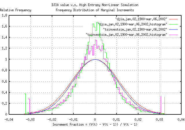
Figure VI is the frequency distribution of the marginal increments of the DJIA's value, from January 2, 1900, to March 6, 2002, and a least squares fit of the distribution to a Normal/Gaussian bell curve distribution. The binomial frequency distribution of the marginal increments of the time series simulated with the tsinvestsim program. The data in Figure VI was made with the tsnormal program.

It has been suggested that the leptokurtosis in economic time series is created by the fractal dimension of the data not being 2- which is the value for a simple Brownian motion fractal-and persistence, (i.e., a slight tendency for the next movement in the time series to be like the last.) But there can be other reasoning, too.

    tsmath -l djia1900-2002 | tslsq -o | tsroot -l | \
        tsscalederivative > djia.1900.jan.02-2002.mar.06
    tsinvestsim -n 1000 data 28048 | tsmath -l | tslsq -o | tsroot -l | \
        tsscalederivative > tsinvestsim.jan.02.1900-mar.06.2002

where the data file is the same as used for Figure VI, above.

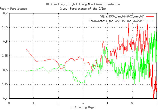
Figure VII is a plot of the persistence, (sometimes called the Hurst Exponent from rescaled range analysis, Range/Scale,) of the DJIA, and a simulation with similar statistics. Of interest is the variability of the persistence-it is far from constant over time, which would be expected in a well behaved fractal. Some observations:

1. The persistence of the DJIA at e^0.693147 = 1 day is 0.573078, and then falls rapidly-this is a contradiction with the Efficient Market Hypothesis, (EMH), which predicates that the market responds to information instantaneously; the contradiction is not serious for most analysis, and the approximation used in the EMH is probably reasonable for general purposes, (all it says is that an instantaneous market response to new information means within a few days.)

2. At about e^2.2 = 9 days, the persistence drops to just over 0.5.

3. And then the persistence raises to about 0.6 through the rest of a calendar year, (of about 253 trading days in a calendar year, or at ln (253) = 5.5, when it, quite quickly, goes anti-persistent.

Although such variability in persistence could be attributed to Non-Linear Dynamical System, (NLDS,) dynamics, it is more likely a structural artifact. For example, the anomaly could be created by a downtrend, followed by an uptrend about 30 trading days later, on average, that happens, on average, about once a year, (in addition to the short term few day inefficiency.) Looking at the time series of the DJIA, October and November frequently have about a month and a half downward spike, which also happens to correspond with October 31, the time that mutual fund capital and income gains taxation liabilities are executed at the end of the fiscal year, as mandated under US Federal law, (usually, resulting in mutual fund companies holding a fire sale on equities they hold with bad pro forma.) Note, also, that many NLDS methodologies would indicate that structural phenomena are system dynamics-leading to inappropriate interpretations of the data.

However, using an average persistence of 0.57 for the DJIA, (and its constituent equities, too,) can adequately model the NLDS/structural phenomena. This means that the root-mean-square of the marginal increments, rms, would not be added as ((1 / n) * sum increment^2)^0.5, but as ((1 / n) * sum increment^(1 / 0.57))^0.57. (For an example of the consequences of assuming that risk is represented as the root-mean-square of the marginal increments, see the section on the DJIA, from Section III.

Of passing interest is the fact that, as shown in Figure VII, the simulation showed substantial leptokurtosis, but no persistence.

Appendix I, Useful Approximations

As a approximation for non-linear high entropy economic system's daily data, from Equation (1.20), the exponential marginal gain per unit time, g, will typically be about 1.0002, and the ln (1.0002) will be about 0.0002. The average of the time series' marginal increments, avg, that has exponential marginal gain per unit time, g = 1.0002 will be about 0.0004. So, as an approximation, divide the avg by two, and that's the ln (g); add unity to get g.

If a non-linear high entropy economic system is assummed to be operating near optimality-a reasonable assumption for most economic systems-then substituting Equation (1.26) into Equation (1.24):

    avg
    ---- + 1
    rms         rms + 1   sqrt (avg) + 1
    --------  = ------- = -------------- ...............(1.31)
       2           2            2

--

John Conover, john@email.johncon.com, http://www.johncon.com/