|
From: John Conover <john@email.johncon.com>
Subject: Quantitative Analysis of Non-Linear High Entropy Economic Systems V
Date: 14 Feb 2002 07:38:46 -0000
As mentioned in Section I, Section II, Section III and Section IV much of applied economics has to address non-linear high entropy systems-those systems characterized by random fluctuations over time-such as net wealth, equity prices, gross domestic product, industrial markets, etc.
The dynamics of non-linear high entropy systems are probabilistic in nature, and the understanding of the mathematics involved permits engineered solutions in the field of finance, such as development of strategies for portfolio growth optimization.
Note: the C source code to all programs used is available from the NtropiX Utilities page, or, the NdustriX Utilities page, and is distributed under License.
As a demonstration of financial engineering, a simple portfolio management strategy will be developed. From Section I, Important Formulas, Equation (1.24):
        avg
        --- + 1
        rms
    P = ------- ........................................(1.24)
           2
where avg and
avg are the average and deviation of the
marginal increments, respectively, and P
is the likelihood of an up movement in the price of an equity. From Equation
(1.20):
                 P          (1 - P)
    g = (1 + rms)  (1 - rms)        ....................(1.20)
g is the average increase in price of
an equity per unit time, for example, after
n many days, an equity's value would
have increased in value by a factor of
g^n.
Equation
(1.24) and Equation
(1.20) work on a portfolio's value, too. Let
avgp and
rmsp be the average and the deviation of
the marginal increments of the portfolio's value, and
Pp be the the likelihood of an up
movement in the portfolio's value. Then:
         avgp
         ---- + 1
         rmsp
    Pp = ------- ........................................(5.1)
           2
and:
                   Pp           (1 - Pp)
    gp = (1 + rmsp)   (1 - rmsp)         ................(5.2)
where gp is the average increase in
value of the portfolio per unit time.
To increase gp,
Pp must increase, and, to increase
Pp, avgp
must increase, and/or, rmsp
decrease.
Knowing that for avg << rms,
the averages of the marginal increments of the equities in a portfolio
add linearly:
           1         1               1
    avgp = -  avg  + -  avg  + ... + -  avg  ............(5.3)
           K     1   K     2         K     K
            1         2               2     n
where the subscripts denote the avg
of the n individual equities in the
portfolio, and K is the fraction of the
portfolio allocated to an individual equity.
Knowing that for avg << rms,
deviations of the fluctuations in equity prices add root-mean-square
in the portfolio:
                  1      2     1      2
    rmsp = sqrt ((-  rms  ) + (-  rms  )  + ...
                  K     1      K     2
                   1            2

                  1      2
           ... + (-  rms  )) ............................(5.4)
                  K     n
                   n
The median values of the daily average and deviation of the
marginal increments of equities on the US exchanges, avg
= 0.0004 and rms = 0.02,
respectively, can be used as an approximation for all equities in the
portfolio to simplify the equations:
1 1 1
avgp = - avg + - avg + ... + - avg ...............(5.5)
n n n
= avg
since there are n many of terms, and:
1 2 1 2
rmsp = sqrt ((- rms ) + (- rms ) + ...
n n
1 2
... + (- rms )) .............................(5.6)
n
1
= -------- rms
sqrt (n)
since there are n many of terms.
|
|
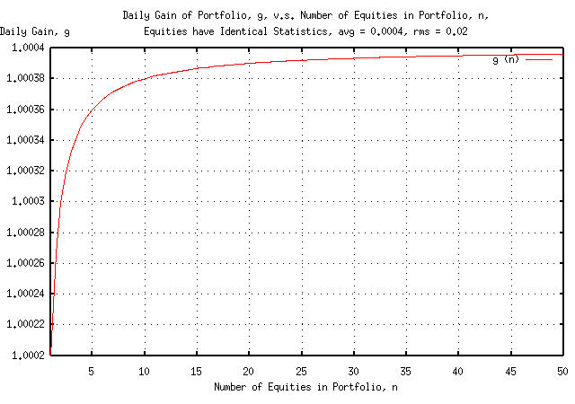
Figure I is a plot of the average daily gain,
g of a portfolio consisting of
n many identical equities, each having
an average and deviation of the marginal increments of its price,
avg = 0.0004, and rms =
0.02, respectively, with equal asset allocation.
Of interest is that the average daily gain,
g, of the portfolio can be almost
doubled, (which is what we set out to do,) by maintaining an equal
asset allocation in the equities in the portfolio-but the marginal
utility of more than ten assets diminishes rapidly.
The simple portfolio management strategy:
Always maintain about ten equities in the portfolio.
Always maintain about equal asset allocation between the ten equities.
|
As a side bar, the simple portfolio management strategy is not new. From "Reuter", April 27, 1997, Peter Lynch was quoted as saying: Investors should ... take time to research five to 10 companies ... buy good firms and hold the stock for the long run ... As a generalization, the strategy is used as a context by fund managers, (most funds average about 10 equities in the portfolio, and maintain about equal asset allocations, over the long run.) However, most funds use mathematical programming for precise adjust of allocations, and will juggle asset allocations with the mood of the time. For example, adjusting allocations for equal risk, (the
deviation of the marginal increments of an equity's price,
equal for all For less volatile times, Equation (1.18), from Section I, Important Formulas, can be used: A reasonable approximation to Equation
(1.18) is when the asset allocation for all
If it is assumed, as an approximation, that There is an interesting corollary to all this-it is possible to make money on equities that are decreasing in price without going short, or doing puts. Setting the average multiplicative gain per iteration of the
game, for an equity to have a positive gain in value. The
implication is that an equity's gain in value can be
negative, even though the likelihood of an up movement in the
value is greater than 50%, and, the average, (e.g., median,)
growth per day, It may seem counter intuitive, but just because the average daily gain in value of an equity is greater than zero, and, the equity's value moves up more than it does down, is not sufficient evidence that the equity's value will increase, (e.g., be a good investment.) Is it a mathematical curiosity, or do we really see equities with these kinds of price characteristics? In fact, the answer is that we do. During the up side of the bubble in high-technology equities of the 1990's, about half of the equities had these characteristics; many were to fall the hardest, too. To explore further, it is recommended that something like the
for 100,000 days, and use the -D 0 -M 0 -m 0 options for The simulation is quite surprising; even though it is a
manufactured data set, the portfolio value increases quite
nicely, even though the equities at the end of the simulation
have virtually zero value-the portfolio made money on equities
that declined in value enough to be virtually worthless. (If one
is skeptical-and one should be-and wants to try it on real data,
there is a file supplied with the Its a very compelling example on the utility of balancing one's portfolio. As a concluding remark to this side bar, there is a remaining
question; what makes a company's equity pro forma
suboptimal-where The answer is greed, (or in Greenspan-speak,
irrational
exuberance,) which turns speculative investing into a
pyramid scheme. The statistic "We have met the enemy and he is us." The investors are the ones that paid more for companies than they were worth. No one else, (and the phenomena is not new or unique, for example, see Extraordinary Popular Delusions And The Madness Of Crowds, 1841.) The market, (that's us,) set the value of the equities, not the market makers and CEOs. We should have known better, (or at least we should have known how to make money-and keep it-exploiting the bubble; which is what this side bar is all about.) |
As an approximation, from above, we also know that our investment horizon should be about a calendar year in the future. But what about the past? How long should we wait to invest in an equity?
From Appendix
I, Quantitative
Analysis of Non-Linear High Entropy Economic Systems Addendum for
a typical, (i.e., median value,) equity on the US markets
which has a median and deviation of the marginal increments of,
avg = 0.0004 and rms =
0.02, respectively, has metrics that will converge on
the average, avg, as a function of
0.02 * erf (1 / sqrt (t)), which is
approximately 0.02 * (1 / sqrt (t)) for
n >> 1 for
t many days in the time series, and the
deviation of the error in the measurement of
avg will be (rms / avg) /
sqrt (t).
|
As a side bar, what is being considered here is very subtle. The market determines the value of an equity. Its like using equity prices as a measuring device, (or metric,) for the value of a company. But the measuring device has stochastic errors as the market responds to information, sometimes under correcting, sometimes over correcting. The market's response determining the price of the equity, is serial on sequence of the information, moving the price as estimated by the market-that's why equity prices are stochastic. Its a consequence of the Efficient Market Hypothesis, (EMH). If the information occurs randomly, (which apparently it
does-there seems to be a limit on the accuracy of prediction of
such things as future dividends for P/E ratios,) then it would
be expected that duration of fluctuations in equity prices
follows an The market determination of the value of a company, and thus its fair market equity price, is very similar to convergence in Bernoulli P Trials, which has similar characteristics-at least as far Brownian motion/random walk equivalent of an equity's price goes. Its as if the aggregate, (whatever that is,) of the market is used as test equipment which has measuring errors. |
Suppose that we want the total probability that an equity
price will move up on any given day. For the typical
characteristics, i.e., a median and deviation of the marginal
increments of, avg = 0.0004 and
rms =
0.02
, respectively, then from Section
I, Important
Formulas, Equation
(1.24):
avg 0.0004
--- + 1 ------ + 1
rms 0.02
P = ------- = ---------- = 0.51.....................(1.24)
2 2
And, letting Pc be the corresponding
probability of the number of standard deviations in the error of the
measurement of avg, (one standard
deviation is approximately 0.02 * (1 / sqrt
(t)).) Then the total probability of an up movement,
compensated for data set size would be P *
Pc, which must be greater than 0.5 for a worthwhile
investment. So, all we have to do is find out how many standard
deviations, 0.02 * (1 / sqrt (t)), are
equal to avg, look up what probability
that is, and use that for Pc.
Working backwards through the numbers for a single equity,
P * Pc = 0.5 = 0.51 * Pc, or
Pc = 0.980392157, and the probability of
an up movement in the equity, compensated for data set size, would be
0.5, and the compensated avg = 0,
meaning that playing this strategy would yield zero gain. But
0.980392157 is 2.06 standard deviations,
and the deviation of the error in the measurement of
avg has to be at least that good.
So, for the compensated avg to be
zero, 2.06 standard deviations of 0.02 * (1 / sqrt
(t)) per standard deviation has to equal
avg =
      0.0004
, or where
0.0004 / 2.06 = 0.02 / sqrt (t), which
means t = 10609 trading days, which is
about 42 years at 253 trading days per calendar year, which is
obviously not a workable solution in light of the durability
of US companies from Section
IV.
However, suppose we construct a portfolio of ten equities. Then how long should we wait to invest in an equity?
Doing the same thing:
                  avg
        sqrt (10) --- + 1
                  rms
    P = ----------------- = 0.5316227766 ...............(1.24)
                2
And, again, working backwards through the numbers for the
portfolio of ten statistically similar equities, (assuming the equity
prices are statistically independent,) P * Pc = 0.5 =
0.5316227766 * Pc, or Pc =
0.940516513, and the probability of an up movement in
the equity, compensated for data set size, would be 0.5, and the
compensated avg = 0, meaning that
playing this strategy would yield zero gain. But
0.940516513 is 1.555 standard
deviations, and the deviation of the error in the measurement of
avg has to be at least that good.
So, for the compensated avg to be
zero, 1.555 standard deviations, of (0.02 / sqrt (10)) *
(1 / sqrt (t)) per standard deviation, has to equal
avg = 0.0004, or where
0.0004 / 1.555 = (0.02 / sqrt (10)) * (1 / sqrt
(t))
, which means t =
605 trading days, which is about 2.4 years at 253
trading days per calendar year-a much more workable scenario.
Note that 2.4 years is the minimum; buying equities with less than a 2.4 year history, and one would, eventually, lose all one's money, (as many did in the dot-com mania.) Requiring a 4.4 year history of an equity to be listed before investing would be even better-since 4.4 years is the median value of bubbles in equity prices.
Which completes the simple portfolio management strategy:
Always maintain about ten, or more, equities in the portfolio.
Always maintain about equal asset allocation between the ten equities.
Always consider the investment horizon to be about a calendar year.
Always be skeptical of investing in companies with less than a two and a half year history of being a publicly traded-preferably, a minimum of four and a half years.
Note that the simple portfolio management strategy-a financially engineered solution-is nothing more than four simple policies; an investment framework, (that's what financial economics is all about.) The policies are listed in order of importance, and the second policy is the one that makes the money-its the engine of the strategy.
|
As a side bar, the strategy is an equity investment architecture-it does not pick equities, nor does it attempt to time the market. The strategy has been known by professionals for about a half century, and has demonstrated flexibility and performance advantages. The strategy is really a spin on Black-Scholes-Merton options trading strategies, which has an outstanding performance history. Why don't more people know about it? Few have the intellectual tenacity to struggle through the abstract mathematical models, which are axiomatic, and sometimes counter intuitive to many. The strategy can be beat, in the short run, (50% of the time, for less than 4.4 years,) on shear luck alone-but in the long run, it is very difficult to do better. (For example, it was beat during the dot-com upside quite significantly; but in the long run-including the dot-com crash-it did quite well, overall. |
How well does the simple portfolio management strategy work?
To find out, the price history of the first ten equities, (in alphabetical order,) in the DJIA were downloaded from Yahoo!'s Historical Prices database, (the prices are adjusted for splits,) and the investment strategy simulated. The simulation is to simply to maintain equal asset allocation, in each of the ten equities, every day, and the annual returns measured. Since, by luck alone, any strategy-no matter how irrelevant-could show good returns for 4.4 years, 50% of the time, (that's the implication of Equation 3.2,) the simulation will consist of a quarter of a century of daily returns.
The construction of the simulation with the historical data is outlined in Appendix I, for those so inclined.
|
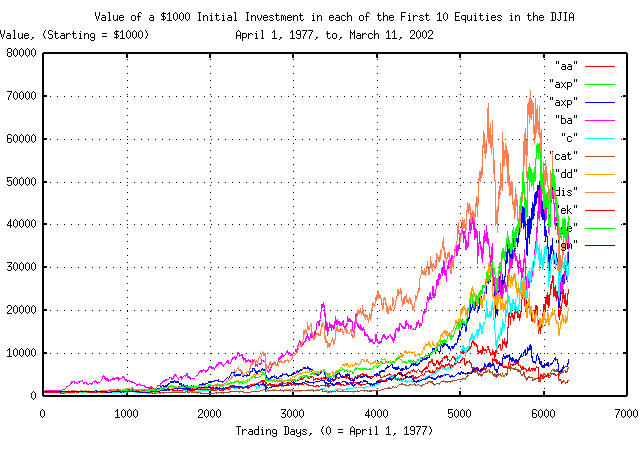
Figure II is a plot of the pro forma of the individual equities picked from the DJIA, by ticker symbol. Each equity started with an initial investment of $1000. The plot represents the growth in value of a portfolio consisting of exactly one equity, with an initial investment of $1000, held for a quarter of a century. It will be used for comparative purposes.
|
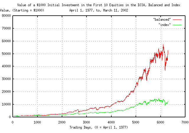
Figure III is a plot of the index value of the same ten equities picked from the DJIA, and the result of balancing the asset allocation between the ten equities, equally, every day, for a quarter of a century, starting with an initial investment of $1000.
The index graph represents the pro forma of a portfolio with an initial investment of $1000, a quarter of a century ago, in the ten equities, and then just letting the investment ride.
The balanced graph represents the pro forma of a portfolio with an initial investment of $1000, a quarter of a century ago, in the same ten equities, but the asset allocation between the equities was made equal, each, and every day.
And, how did it work out?
The simple portfolio management strategy:
Increased the portfolio value faster than the value of any equity in the portfolio.
Beat the index of all equities in the portfolio.
The particulars:
The equity value with the fastest growth, over the quarter of a century, was GE, which increased in value by a factor of 41.56566, (about 16.1% per year.) The simple portfolio management strategy increased the portfolio value by a factor of 52.68776, (about 17.2% per year,) resulting in a 26.757905444% improvement in the quarter century investment over any single equity, (i.e., the simple portfolio management strategy grew the value of the portfolio faster than the value any equity in the portfolio grew, which is in line with theoretical expectations.)
The index value of the ten equities, (i.e., the summed value of the equities,) increased by a factor of 12.655270655 for the quarter century-about 10.7% per year vs. the 17.2% for the simple portfolio management strategy, (which is reasonably near the theoretical expectations of about 2X.) The simple portfolio management strategy beat the index by about 4.1633056642-about 4X = 400%-over the quarter century.
|
As a side bar, the simple portfolio management strategy performed well because it mitigated risk-which is often overlooked by investors. The time period of the simulated investment included two bear market downturns/adjustments, (October of 1987 and 1999-2001,) and performed well. Risk management is an important part of financial engineering. Given enough time, no matter how small the risk, sooner or later, it will bite. A portfolio's value can not remain a fugitive from the laws of probability indefinitely. Although the simulation balanced the portfolio every day, this is really not necessary for the casual long term investor. Many balance periodically-once a week, or once a month. Others balance asset allocations when one asset's value exceeds the others by 5-10%. What is necessary is to not have too much of the portfolio's value dependent on a single asset, making the portfolio's value vulnerable to fluctuations in the value of a single investment. Although, through most of the quarter century simulation, at any one time, there was at least one equity that out performed the simple portfolio management strategy, in the long run, the strategy out performed all equities in the portfolio. The metric of risk is the deviation of the marginal increments in an investment's value-i.e., how large the fluctuations in value are. One can look at the graphs, above, and see how the simple portfolio management strategy worked-it was a hedging strategy; the value of each investment in the portfolio was hedged against the combined value of all the others, reducing the fluctuations in the value of the portfolio, visibly. When one equity increased in value more than the others, money was removed from the investment, and re-invested in all the others. The strategy, dynamically, siphons off the gains from the winners at any one time, and defends the gains through investment diversification. Almost all hedging strategies work that way. |
What are the chances of a company funded by a venture capitalist being a high value asset after five years?
Although the log-normal characteristics of a venture capital fund can be computed analytically[1] using the techniques outlined in Section II, simulation has the advantage of developing intuition.
The marginal increments of a typical equity's growth in value has
an average and deviation, avg = 0.0004,
and, rms = 0.02, respectively, which are
the the median values for equities listed on the US markets for the
Twentieth Century. Choosing 1,000 companies to get an adequate
statistical distribution, and identical statistics for all companies,
a tsinvestsim
program data file, sim, would
look like:
    0, p = 0.51, i = 10000000
    1, p = 0.51, i = 10000000
    .
    .
    .
    998, p = 0.51, i = 10000000
    999, p = 0.51, i = 10000000
where, from Equation (1.24):
        avg        0.02
        --- + 1   ------ + 1
        rms       0.0004
    P = ------- = ---------- = 0.51 ....................(1.24)
           2          2
and the companies are numbered, 0, 1, ... 998,
999, with an equal initial investment of ten million
dollars in each company-which was a typical value in the 1990's:
tsinvestsim sim 1265 | tail -1000 | cut -f3 | sort -n > value
where the simulation ran for five calendar years, of 253 working
days per calendar year, 5 * 253 =
1265. The value of the 1,000 companies, at the end of
five years is numerically sorted, smallest value to largest value.
|
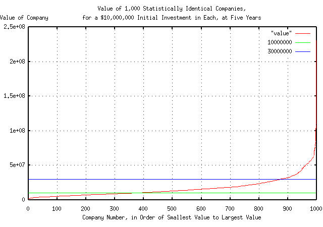
Figure IV is a plot of the simulated values of 1,000 companies,
each with identical statistics, and each with an initial investment of
$10,000,000, after five years. The companies are sorted by value,
least, to most, and numbered, 0, 1, ... 998,
999. This graph is compared with the initial
investment in each company of $10,000,000, and the VC rule-of-thumb
that a company should be able to show at least a factor of three
increase in value in five years to be a desirable investment.
In the simulation, about 40% of the companies lost money, about half met the factor of three requirement, and about 10% were star performers. Note that a fund would be carried by less than 10% of the investment assets-about 1 in 12 is the empirical value for the VC industry, as a whole; that is why it is considered high-risk investing.
|
As a side bar, the graph in Figure IV was relatively stable through the Twentieth Century-from the radio set bubble of the 1930's, to the television set bubble of the 1950's, to the dot-com bubble of the 1990's. It, also, was representative of the bubble'ts of the CB radio, electronic game, semiconductor, and software market expansions in the last quarter of the Century. At the end of the market bubbles, only about one in ten of the companies survived. The rest were acquired, or went out of business, altogether. Those that did survive yielded a factor of slightly more than ten return on investment in the five years, (which is consistent-on the average, in the long run-with Example I, above for a portfolio of ten equities). So, initial investing in start-ups can be lucrative, but one must be prepared for the risks; a nine-out-of-ten failure rate, on average, (or as one cynical VC was quoted as saying when the dot-com bubble burst, you had to kiss nine frogs to get a prince.) |
[1]Computing the equity value of the 90'th percentile companies, for example, working with the Brownian motion/random walk equivalent of the system as described in Section II, and from Equation (2.3), the natural logarithm of the median value of all companies at the end of five years will have increased by:
0.0002 * 1265 = 0.253 ...............................(5.9)
where, the the gain in value, per business day,
g from Equation
(1.20):
                  0.51           (1 - 0.51)
    g = (1 + 0.02)     (1 - 0.02)           = 1.0002 ....(5.10)
has a natural logarithm of ln (1.0002) =
0.0002, and the natural logarithm of the deviation of
the values of all companies in the fifth year, from Equation
(2.4):
0.02 * sqrt (1265) = 0.71133677 .....................(5.11)
The 90'th percentile is about 1.28
deviations, (from the normal probability
function table of values,) so:
    ln (M) = 0.253 + (1.28 * 0.71133677)

           = 1.16351106528 ..............................(5.12)
Or an increase in value by at least a factor of M =
3.2011530252 is the 90'th percentile in Figure
IV, above, (i.e., 900 companies have less, 100 have more-or one in
nine, on average, will have a market capitalization worth more than
$32,011,530 at the end of five years, based on an initial investment
of $10,000,000.)
The price history for each of the ten equities were downloaded from
Yahoo!'s Historical Prices database, (the
prices are adjusted for splits,) and the csv2tsinvest
program used to convert the price histories from csv spread sheet
format to tsinvest
time series format, for example, for GE's price history:
csv2tsinvest GE ge.csv > ge
There is an issue with the csv spreadsheet data; it is not Y2K compliant, (the years are listed as 77, 78, ... 01, 02,) which was fixed with sed(1), or a text editor could be used to insert "19" before any year not beginning with 0, else, insert 20.
The tsinvest
time series for all equities were combined using the sort(1) command,
to make a combined time series of all equities,
djia, (which is why the date/time stamp
is the first column of a tsinvest
database.)
The tsinvest
program was used for the simulations:
    tsinvest -D 0 -m 10 -M 10 -i djia | cut -f1 > balanced
    tsinvest -D 0 -m 10 -M 10 -i -j djia | cut -f1 > index
The Unix cut(1) command was used to cut all except the first column
of the tsinvest
output file, which is the index, (that's all we are interested in for
this simulation.) The -D 0,
-m 0, and, -M
0 options shut down any optimization that the tsinvest
program would normally make, (they tell the program to unconditionally
invest in an equity, whether it normally would, or not, and, in no
less than 10 equities at any one time, and no more than 10-i.e., no
matter what, invest in the 10 equities.) The
-i option tells the program to produce
an index-which by default is always balanced for comparison with the
other strategies that the program is capable of-and the
-i tells the program to not to balance
the index values.) The files balanced
and index were then plotted.
The tsmath
program was used to multiply a tsinvest
time series to adjust for an initial investment of $1000 for plotting
comparisons of the individual equities, which were then plotted.
--

John Conover, john@email.johncon.com, http://www.johncon.com/