|
From: John Conover <john@email.johncon.com>
Subject: Quantitative Analysis of Non-Linear High Entropy Economic Systems IV
Date: 14 Feb 2002 07:38:46 -0000
As mentioned in Section I, Section II and Section III, much of applied economics has to address non-linear high entropy systems-those systems characterized by random fluctuations over time-such as net wealth, equity prices, gross domestic product, industrial markets, etc.
The dynamics of non-linear high entropy systems are probabilistic in nature, and require a suitable methodology for analysis.
Note: the C source code to all programs used is available from the NtropiX Utilities page, or, the NdustriX Utilities page, and is distributed under License.
The file
ge.jan.02.1962-mar.1.2002
contains the time series of GE's daily close equity price history,
from January 2, 1962, through, March 2, 2002, (10,113 days,)
inclusive. The data is from Yahoo!'s Historical Prices database, and
is adjusted for splits.
The file was converted to a Unix flat file database with the csv2tsinvest
program:
csv2tsinvest GE ge.csv > ge.jan.02.1962-mar.1.2002
Analysis:
Analyzing the time series for the GE equity price time series:
    tsfraction ge.jan.02.1962-mar.1.2002 | tsavg -p
    0.000507

    tsfraction ge.jan.02.1962-mar.1.2002 | tsrms -p
    0.015451

    tsgain -p ge.jan.02.1962-mar.1.2002
    1.00038773455
where the average of the marginal incrments, avg =
0.000507, the root-mean-square of the marginal
increments, rms = 0.015451, and the gain
of the marginal increments, g, and:
        avg       0.000507
        --- + 1   -------- + 1
        rms       0.015451
    P = ------- = ------------ = 0.51640670507 .........(1.24)
           2           2
are used in the file, sim,
which contains the single record:
GE, p = 0.51640670507, f = 0.015451
and making the simulation file for GE equity price:
tsinvestsim sim 10113 > ge.jan.02.1962-mar.1.2002.tsinvestsim
where the file,
ge.jan.02.1962-mar.1.2002.tsinvestsim
is the simulated GE equity price time series with identical
statistics.
The value of the variables will be used in analysis of the dynamics
of GE's equity price, a non-linear high entropy economic system, by
comparing the dynamics of the empirical data with the dynamics of both
the simulated data and its theoretical abstraction,
constant * erf (1 / sqrt (t)).
The file
ge.jan.02.1962-mar.1.2002
contains the time series of GE's daily close equity price history,
from January 2, 1962, through, March 2, 2002, (10,113 days,)
inclusive. The data is from Yahoo!'s Historical Prices database, and
is adjusted for splits.
The file was converted to a Unix flat file database with the csv2tsinvest
program:
csv2tsinvest GE ge.csv > ge.jan.02.1962-mar.1.2002
The cumulative probability of the duration of the increases and
decreases in the average of the marginal increments,
avg, of GE's equity price:
    #!/bin/sh

    interval=1

    while [ $interval -le 4048 ]
    do

        tsmath -l ge.jan.02.1962-mar.1.2002 | tslsq -o | \
            tsderivative | tsavgwindow -w $interval | tsrms -p >> \
            ge.jan.02.1962-mar.1.2002.avgwindow

        tsmath -l ge.jan.02.1962-mar.1.2002.tsinvestsim | tslsq -o | \
            tsderivative | tsavgwindow -w $interval | tsrms -p >> \
            ge.jan.02.1962-mar.1.2002.tsinvestsim.avgwindow

        interval=`expr $interval + 1`

    done
which uses the tsavgwindow
program to calculate the average of the marginal increments over the
time interval, interval, for all
intervals from 1 to
4048, and the tsrms
program to calculate the deviation of the average, for GE's equity
price.
|
|
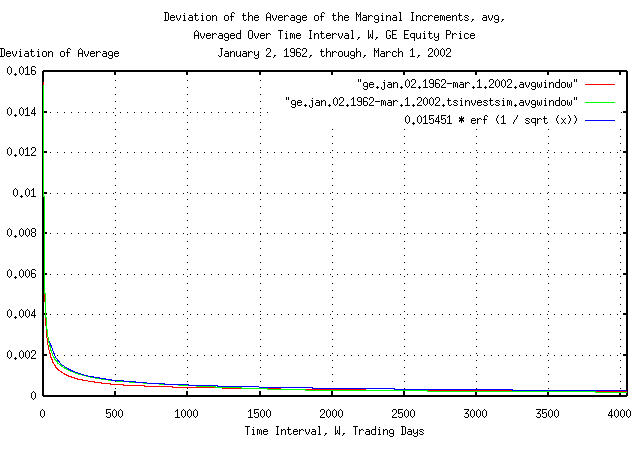
Figure I is a plot of the cumulative probability of the duration of
the increases and decreases in the average of the marginal increments,
avg, of GE's equity price, and its
simulation, with the theoretical value, 0.015451 * erf
(1 / sqrt (t)). The frequency of the durations of the
increases and decreases of up to 4,048 trading days, (about 16
calendar years,) are shown.
|
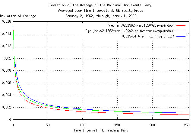
Figure II is a plot of the cumulative probability of the duration
of the increases and decreases in the average of the marginal
increments, avg, of GE's equity price,
and its simulation, with the theoretical value, 0.015451
* erf (1 / sqrt (t)). The frequency of the durations
of the increases and decreases of up to 253 trading days, (about a
calendar year,) are shown. Figure II the same as Figure I, but shows
only the frequency of short durations of increases and decreases for
clarity.
|
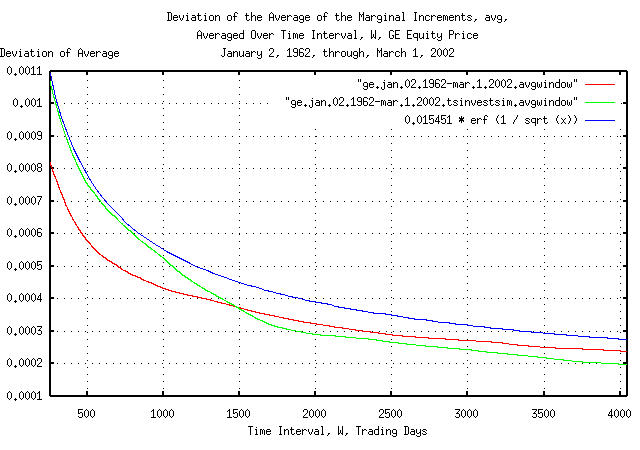
Figure III is a plot of the cumulative probability of the duration
of the increases and decreases in the average of the marginal
increments, avg, of GE's equity price,
and its simulation, with the theoretical value, 0.015451
* erf (1 / sqrt (t)). The frequency of the durations
of the increases and decreases of 253 trading days, (about a calendar
year,) to 4,048 trading days, (about 16 calendar years,) are shown.
Figure III is the same as Figure I, but shows only the frequency of
long durations of increases and decreases for clarity. Since the data
set size consisted of only 10,113 trading days, the empirical
cumulative probability is smaller than the theoretical value by
0.015451 * erf (1 / sqrt (10113)) = 0.015451 * 0.011968
= 0.000184917568
at 4,048 trading days.
Figures I, II, and III, are the cumulative probability of the
duration of the increases and decreases in the average of the marginal
increments, avg, of GE's equity
price. For example, at the end of any 500 trading day interval, (about
2 calendar years,) the average of the marginal increments would be
within about, plus, or minus, 0.0008 of
its mean value of 0.000507 for one
standard deviation, about 68%, of the time.
The cumulative probability of the duration of the increases and
decreases in the deviation of the marginal increments,
rms, of GE's equity price:
    #!/bin/sh

    interval=1

    while [ $interval -le 4048 ]
    do

        tsmath -l ge.jan.02.1962-mar.1.2002 | tslsq -o | \
            tsderivative | tsrmswindow -w $interval | tsmath -s 0.015451 | tsrms -p >> \
            ge.jan.02.1962-mar.1.2002.rmswindow

        tsmath -l ge.jan.02.1962-mar.1.2002.tsinvestsim | tslsq -o | \
            tsderivative | tsrmswindow -w $interval | tsmath -s 0.015451 | tsrms -p >> \
            ge.jan.02.1962-mar.1.2002.tsinvestsim.rmswindow

        interval=`expr $interval + 1`

    done
which uses the tsrmswindow
program to calculate the deviation of the marginal increments over the
time interval, interval, for all
intervals from 1 to
4048, the tsmath
program to subtract the mean value of the deviation of the marginal
increments, rms, and the tsrms
program to calculate the deviation of the deviation for GE's equity
price.
|
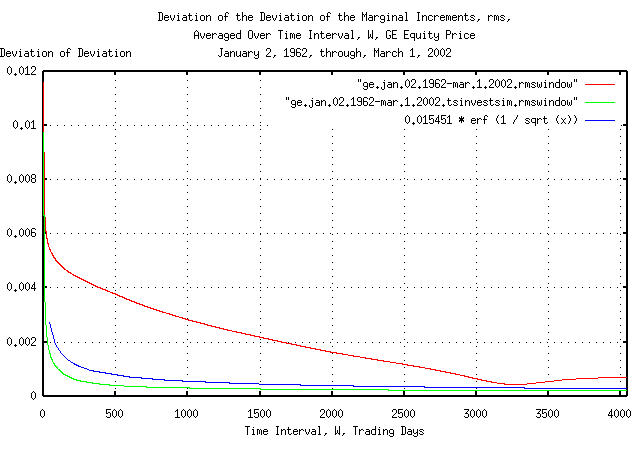
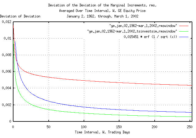
Figure IV is a plot of the cumulative probability of the duration
of the increases and decreases in the deviation of the marginal
increments, rms, of GE's equity price,
and its simulation, with the theoretical value, 0.015451
* erf (1 / sqrt (t)). The frequency of the durations
of the increases and decreases of up to 4,048 trading days, (about 16
calendar years,) are shown.
The apparent discrepancy between the empirical and theoretical values of the cumulative probability of the duration of the increases and decreases in the deviation of the marginal increments is an artifact of the interaction between the windowing construct used for measuring the deviation over time intervals and a 13 year cyclic clustering phenomena in the time series. See Appendix I for particulars.
|
Figure V is a plot of the cumulative probability of the duration of
the increases and decreases in the deviation of the marginal
increments, rms, of GE's equity price,
and its simulation, with the theoretical value, 0.015451
* erf (1 / sqrt (t)). The frequency of the durations
of the increases and decreases of up to 253 trading days, (about a
calendar year,) are shown. Figure V the same as Figure IV, but shows
only the frequency of short durations of increases and decreases for
clarity.
|
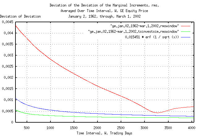
Figure VI is a plot of the cumulative probability of the duration
of the increases and decreases in the deviation of the marginal
increments, rms, of GE's equity price,
and its simulation, with the theoretical value, 0.015451
* erf (1 / sqrt (t)). The frequency of the durations
of the increases and decreases of 253 trading days, (about a calendar
year,) to 4,048 trading days, (about 16 calendar years,) are shown.
Figure VI is the same as Figure IV, but shows only the frequency of
long durations of increases and decreases for clarity. Since the data
set size consisted of only 10,113 trading days, the empirical
cumulative probability is smaller than the theoretical value by
0.015451 * erf (1 / sqrt (10113)) = 0.015451 * 0.011968
= 0.000184917568
at 4,048 trading days.
Figures IV, V, and VI, are the cumulative probability of the
duration of the increases and decreases in the deviation of the
marginal increments, rms, of GE's equity
price. For example, at the end of any 500 trading day interval, (about
2 calendar years,) the deviation of the marginal increments would be
within about, plus, or minus, 0.00075 of
its mean value of 0.015451 for one
standard deviation, about 68%, of the time.
The cumulative probability of the duration of the increases and
decreases in the likelihood of an up movement in the marginal
increments, P, of GE's equity price:
    #!/bin/sh

    interval=1

    while [ $interval -le 4048 ]
    do

        tsshannonwindow -a -w $interval ge.jan.02.1962-mar.1.2002 | \
            tsmath -s 0.51640670507 | tsrms -p >> ge.jan.02.1962-mar.1.2002.Pwindow

        tsshannonwindow -a -w $interval ge.jan.02.1962-mar.1.2002.tsinvestsim | \
            tsmath -s 0.51640670507 | tsrms -p >> ge.jan.02.1962-mar.1.2002.tsinvestsim.Pwindow

        interval=`expr $interval + 1`

    done
which uses the tsshannonwindow
program to calculate the likelihood of an up movement,
P, of the marginal increments over the
time interval, interval, for all
intervals from 1 to
4048, the tsmath
program to subtract the mean value of the likelihood of an up movement
of the marginal increments, P, and the
tsrms
program to calculate the deviation of the likelihood of an up movement
of the marginal increments.
|
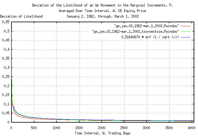
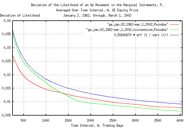
Figure VII is a plot of the cumulative probability of the duration
of the increases and decreases in the likelihood of an up movement in
the marginal increments, P, of GE's
equity price, and its simulation, with the theoretical value,
0.51640670507 * erf (1 / sqrt (t)). The
frequency of the durations of the increases and decreases of up to
4,048 trading days, (about 16 calendar years,) are shown.
|
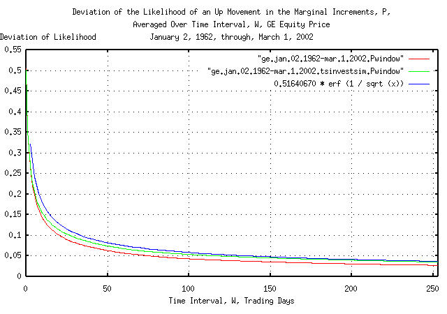
Figure VIII is a plot of the cumulative probability of the duration
of the increases and decreases in the likelihood of an up movement in
the marginal increments, P, of GE's
equity price, and its simulation, with the theoretical value,
0.51640670507 * erf (1 / sqrt (t)). The
frequency of the durations of the increases and decreases of up to 253
trading days, (about a calendar year,) are shown. Figure VIII the same
as Figure VII, but shows only the frequency of short durations of
increases and decreases for clarity.
|
Figure IX is a plot of the cumulative probability of the duration
of the increases and decreases in the likelihood of an up movement in
the marginal increments, P, of GE's
equity price, and its simulation, with the theoretical value,
0.51640670507 * erf (1 / sqrt (t)). The
frequency of the durations of the increases and decreases of 253
trading days, (about a calendar year,) to 4,048 trading days, (about
16 calendar years,) are shown. Figure IX is the same as Figure VII,
but shows only the frequency of long durations of increases and
decreases for clarity. Since the data set size consisted of only
10,113 trading days, the empirical cumulative probability is smaller
than the theoretical value by 0.51640670507 * erf (1 /
sqrt (10113)) = 0.51640670507 * 0.011968 =
0.00618035545 at 4,048 trading days.
Figures VII, VIII, and IX, are the cumulative probability of the
duration of the increases and decreases in the likelihood of an up
movement in the marginal increments, P,
of GE's equity price. For example, at the end of any 500 trading day
interval, (about 2 calendar years,) the likelihood of an up movement
in the marginal increments would be within about, plus, or minus,
0.025 of its mean value of
0.51640670507 for one standard
deviation, about 68%, of the time.
The cumulative probability of the duration of the increases and
decreases in the gain of the marginal increments,
g, of GE's equity price:
    #!/bin/sh

    interval=1

    while [ $interval -le 4048 ]
    do

        tsgainwindow -w $interval ge.jan.02.1962-mar.1.2002 | \
            tsmath -s 1.00038773455 | tsrms -p >> ge.jan.02.1962-mar.1.2002.gwindow

        tsgainwindow -w $interval ge.jan.02.1962-mar.1.2002.tsinvestsim | \
            tsmath -s 1.00038773455 | tsrms -p >> ge.jan.02.1962-mar.1.2002.tsinvestsim.gwindow

        interval=`expr $interval + 1`

    done
which uses the tsgainwindow
program to calculate the gain, g, of the
marginal increments over the time interval,
interval, for all intervals from
1 to 4048,
the tsmath
program to subtract the mean value of the gain of the marginal
increments, g, and the tsrms
program to calculate the deviation of the gain of the marginal
increments.
|
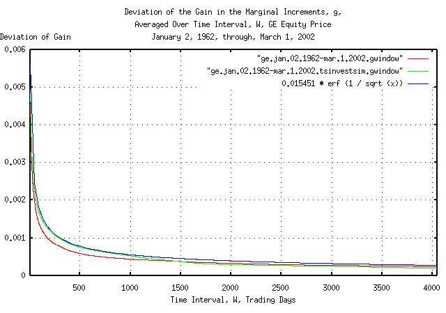
Figure X is a plot of the cumulative probability of the duration of
the increases and decreases in the gain of the marginal increments,
g, of GE's equity price, and its
simulation, with the theoretical value, 0.015451 *
erf (1 / sqrt (t)). The frequency of the durations of
the increases and decreases of up to 4,048 trading days, (about 16
calendar years,) are shown.
|
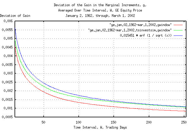
Figure XI is a plot of the cumulative probability of the duration
of the increases and decreases in the gain of the marginal increments,
g, of GE's equity price, and its
simulation, with the theoretical value, 0.015451 * erf
(1 / sqrt (t)). The frequency of the durations of the
increases and decreases of up to 253 trading days, (about a calendar
year,) are shown. Figure XI the same as Figure X, but shows only the
frequency of short durations of increases and decreases for
clarity.
|
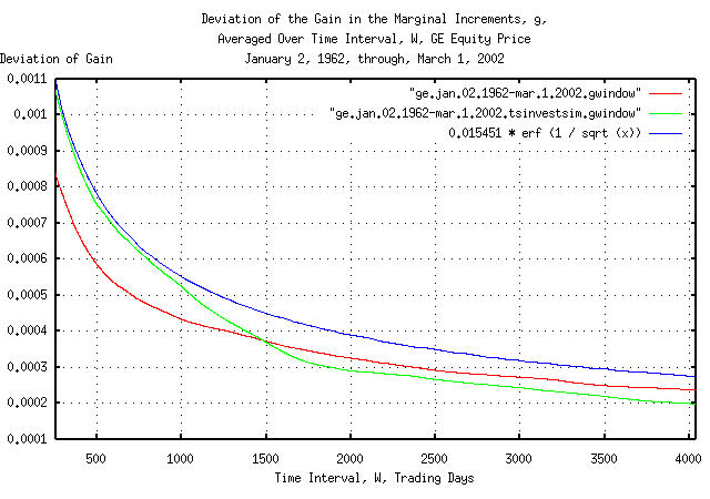
Figure XII is a plot of the cumulative probability of the duration
of the increases and decreases in the gain of the marginal increments,
g, of GE's equity price, and its
simulation, with the theoretical value, 0.015451 * erf
(1 / sqrt (t)). The frequency of the durations of the
increases and decreases of 253 trading days, (about a calendar year,)
to 4,048 trading days, (about 16 calendar years,) are shown. Figure
XII is the same as Figure X, but shows only the frequency of long
durations of increases and decreases for clarity. Since the data set
size consisted of only 10,113 trading days, the empirical cumulative
probability is smaller than the theoretical value by
0.015451 * erf (1 / sqrt (10113)) = 0.015451 * 0.011968
= 0.000184917568
at 4,048 trading days.
Figures X, XI, and XII, are the cumulative probability of the
duration of the increases and decreases in the gain of the marginal
increments, g, of GE's equity price. For
example, at the end of any 500 trading day interval, (about 2 calendar
years,) the gain of the marginal increments would be within about,
plus, or minus, 0.0011 of its mean
value of 1.00038773455 for one standard
deviation, about 68%, of the time.
|
As a side bar, none other than Sir Isacc Newton, referenced in Harvard Magazine's The Damn'd South Sea, was foiled by the dynamics of speculative markets-as were many more recently in the dot-com, (which came to be called the dot-bomb,) market. An equity increasing in price, generously, for two years is no indication that the good fortune will continue. About 16%, one deviation, of the time, it would be expected
that GE's equity gain, That's the good news. The bad news is that at 1,012 trading
days, (or about 2 years later,) the chances that GE's equity
price would still be maintaining the factor of 2 growth in value
would be about |
How much would a typical equity's price on the US exchanges be expected to fluctuate in a year?
From Section III, Equation (3.1):
rms * sqrt (t) .....................................(3.1)
which is a formula for the deviation of the magnitude of
bubbles for the Brownian motion/random walk equivalent of
equity prices. It is, also, the range,
R, often used in Range/Scale,
(Hurst,) analysis.
Converting to log-normal characteristics, the maximum, and minimum, respectively would be:
          +rms * sqrt (t)
    V0 * e                ..............................(4.1)

          -rms * sqrt (t)
    V0 * e                ..............................(4.2)
where rms is the deviation of the
marginal increments in an equity's price,
v0 is the starting value of an equity
price, and t, is some time in the
future.
The median value for the daily marginal increments in an equity
price on the US exchanges is about rms =
0.02, so for t = 253
trading days in a calendar year, a typical equity's minimum
and maximum price would be:
+0.02 * sqrt (253)
V0 * e = 1.37454047383 ...........(4.3a)
-0.02 * sqrt (253)
V0 * e = 0.727515864 .............(4.4a)
A typical equity's price maximum, divided by its minimum,
in a year, will be 1.8893615142, or
about a factor of 2, where
typical means a standard deviation, (i.e., about 68% will be
less, 32%, more.)
Its interesting, because from "Reuter", April 27, 1997, Peter Lynch was quoted as saying:
... Stocks are volatile ... the average stock listed on the New York Stock Exchange fluctuates 50 percent between its annual high and low ...
Although non-linear high entropy economic systems typically exhibit long term exponential growth, that does not mean they can not go bust. An interesting question is how long a public company, on average, is listed on an exchange.
It is a difficult analytical problem because of the discontinuities; companies have different initial public offering equity prices, there are splits which effectively reduce the IPO price, and when a company's equity price falls below one dollar, it is de-listed. Not to mention that companies get de-listed when they are acquired, too.
However, some work on http://www.google.com/ indicated that after adjusting for splits, a reasonable estimate for the median, (half more, half less,) value of the IPO price for US equities in the Twentieth Century was about two dollars.
For the Twentieth Century, the median value, (half more, half
less,) of the average and deviation of the daily marginal increments
in equity prices for those listed on the US exchanges was about
avg = 0.0004, and, rms =
0.02, respectively.
|
As an interesting side bar, from Section I, Equation (1.24), and, Equation (1.18): meaning that most, (actually, the median,) of the equities of US public companies in the Twentieth Century grew maximally optimal. |
The following tsinvestsim
program file, exchange, was
made for 500 companies:
0, p = 0.51, i = 2
1, p = 0.51, i = 2
.
.
.
498, p = 0.51, i = 2
499, p = 0.51, i = 2
where the company names are 0, 1, ... 498,
499 and all the company's stocks are statistically
identical, i.e., they all start at an IPO price of two dollars, and
are maximally optimal with avg = 0.0004,
rms =
0.02
, and P =
0.51.
The C source code to the tsinvestsim
program had to be modified for the simulation so that whenever a
company's equity value dropped below a dollar, it had to be
de-listed. The following construct was added to the tsinvestsim
C source code, version 1.3, dated 2001/12/07 10:05:09, at line
588:
    if (sum < (double) 1.0) /* stock's value less than a buck? */
    {
        sum = (double) 0.0; /* yes, de-list the stock */
        stock->sum = (double) 0.0;
        stock->f = (double) 0.0;
    }
which, if an equity's value is ever less than one dollar, set's it
to zero, forever. A simulation of 5,566 = 22 *
253 trading days, or 22 calendar years of 253 trading
days in a calendar year:
./tsinvestsim exchange 5566 > result
was run, and the last 500 records of the output file,
result, searched for equities with zero
value. There were 206 out of the
500, or
41.2% of the companies had been
de-listed in the 22 calendar year simulation.
The simulation duration of 22 calendar years was chosen because
during the Twentieth Century, the median time a company was listed on
the US exchanges was 22 years. Half were listed for less, half
more. The 41.2% simulation number is
within about 20% of the empirical number. (Although
41% of the companies in the simulation
had failed by 22 years, one had an equity price of
$1333.721702, and the median value of
the 500 equities was $3.207836, compared
with a calculated value of
$3.04430985883 from Section
I, Equation
(1.20). Almost a perfect log-normal distribution.)
|
As a side bar, this is an intuitive result. Using round numbers, during the Twentieth Century a company had a 50% chance of being de-listed every 20 years, or so. So, at the end of 20 years, 50% of the companies would remain. At the end of 40 years, 25% would remain, and at the end of 60, 12.5%, and 6.25% at 80 years, and after a century, 3.125%. There are 30 companies in the DJIA. Of the original that
were in the DJIA in 1900, it would be expected that that
The exponential characteristics of Equation
(1.20) would tend to imply that a company's equity value
would increase forever. That would be true if |
The tsinvestsim
C source code is available in the tsinvest
distribution available from the NtropiX site.
|
As a footnote addendum to this section, (October 19, 2010,) the same is true for the hedge fund industry, too. According to The
Quants: How a New Breed of Math Whizzes Conquered Wall Street
and Nearly Destroyed It, Scott Patterson, Crown Business, a
division of Random House, Inc., New York, New York, 2010, ISBN
978-0-307-45337-2, (which is highly recommended reading,) hedge
funds return, on average, about 20% a year in good times, (to a
one-time maximum as high as 80%.) This means the average and
deviation of the daily marginal increments of a typical hedge
fund would be about where the hedge fund names are A simulation of yields 47.29%, ( The hedge fund industry will have a major "crash" about every 20 years, (the number of fund failures will actually tend to cluster in times of uncertainty,) where about half the hedge funds go out of business. This statistic is supported by the evidence, too. According to A Brief History Of The Hedge Fund by James E. McWhinney, the hedge fund was invented in 1949, with the first crash in 1969-1974, the second 1997-2000, and the third, 2009-2010, for an average of 20 years between hedge fund industry crashes, which is very close to the simulated value, and nearly identical to the durability of US public companies, (See: "The Real Jobs Machine," Robert J. Samuelson, Newsweek, October 11, 2010, pp. 28, which states, "A company founded today has an 80% chance of disappearing over the next quarter century, reports a study by Dane Stangler and Paul Kedrosky of the Kauffman foundation.") This is in reasonable agreement with the theoretical simulations, above, too. Panics, (happening randomly,) on average about every twenty years are an investing inevitability. And, that is true for any non-linear high entropy economic system, including recessions in the GDP, (see: List of recessions in the United States, where the recessions lasting more than one year since the Great Depression are, 1929, 1937, 1973, 1980, and, 2009, which happened, on average, every 20 years,) currency exchange rates, etc. The "mechanism" of the panics is a characteristic of the random process itself-an economic system will experience exponential growth, and sooner or later, the random risks will cluster, overwhelming the exponential growth, and the growth will turn negative for a substantial time-making investing a "deal with the devil." It is similar to a pyramid scheme, where the strategy is to be first-in and first-out. Note the consequences: if one doesn't play, one can't win; but if one plays long enough, one looses. But, doesn't this contradict the paradigm of John Kelly's Kelly criterion? The answer is no. Note that all of the simulations in this
section required a "structural" addition to the |
As a qualitative approximation model, (i.e., simplified
conceptual interpretation for Brownian motion fractals, using the stochastic
calculus, which is not adequate for quantitative
analysis,) the economic system, (equity value, GDP, currency exchange
rate, etc.) is always increasing or decreasing, randomly, (i.e.,
"bubbles," always increasing or decreasing, randomly.) The
probability of a bubble lasting at least
t many years is, approximately,
1 / sqrt (t). For example, the
probability of a positive, (or negative,) parts of the, (Juglar,) business cycle
lasting at least 4 years is 1 / sqrt (4) =
50%, (half of the positive or negative parts of the
business cycles would last less, half more); the chances of a business
cycle "bubble" lasting at least twenty five years would be
1 / sqrt (25) = 20%, and so on. How big
the "bubble" will be, in one year, (if it lasts that long,) is
probabilistic, too, with a standard
deviation of approximately 0.3 * sqrt
(t) for many/most economic systems. For example, 68%
of the time, the economic system movement will be less than +/- 30% in
one year; in four years, less than +/- 60%.
Or, modeling the five positive or negative parts of the business cycles, (each lasting a median of four years, half lasting more, half lasting less,) over an typical 20 year period, one of the business cycles, on average, would have a negative economic system movement of at least a standard deviation, (assuming one out of five is 20% of the time, and is about equal to 16%, which is the the value of the standard deviation-not being precise, this is a simple "thought" model, technically, with a 50% chance,) or a movement of about 60%, which is very close to the 50% loss simulated, above.
Note the simplicity of the economic model-which only assumes that unpredictable things happen to an an economic system, (economy, equity value, etc.,) in a random fashion, which moves the economic system from its current value or state. Once that is assumed, the durability of the economic system is defined by the stochastic calculus.
An analysis of the deviation of the marginal increments of GE's equity price indicates that the deviation is not stable:
    tsmath -l ge.jan.02.1962-mar.1.2002 | tslsq -o | \
        tsderivative | tsrmswindow -w 50 > ge.jan.02.1962-mar.1.2002.rmswindow-50
where the tsrmswindow
program is used to calculate the deviation of the marginal increments
over a moving window of 50 trading
days for GE's equity price.
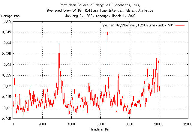
|
Figure XIII is a plot of the deviation, (root-mean-square,) of the
marginal increments, rms, of GE's equity
price, using a 50 trading day moving
window for the calculation of the deviation.
Apparently, there is cyclic phenomena occurring about every
3,300 trading days, (about 13 calendar
years,) causing the calculation of the deviation of the deviation of
the marginal increments of GE's equity price to be too large
everywhere except the dips at
3,300 days in Figure
IV and Figure
VI. The phonomena is quite complex:
| Marginal Increment | Date |
|---|---|
0.066667 |
1962-07-02 |
-0.089744 |
1974-08-23 |
0.070423 |
1974-08-26 |
-0.065789 |
1974-09-04 |
-0.066667 |
1974-09-09 |
0.065574 |
1974-09-16 |
0.088235 |
1974-10-09 |
-0.174757 |
1987-10-19 |
0.082353 |
1987-10-20 |
-0.068293 |
1987-10-22 |
-0.084656 |
1987-10-26 |
0.064426 |
1987-11-05 |
-0.083333 |
1988-01-08 |
-0.106904 |
2001-09-17 |
-0.065502 |
2001-09-20 |
0.124352 |
2001-09-24 |
Note that:
The values are quite large-for example, on 1987-10-19, GE's
equity price suffered a 17.4757% drop
in value; a 0.174757 / 0.015451 =
11.3104006213 deviation incident, which has a
probability of happening that is indistinguishable from zero-yet it
did happen.
The large excursions in high volatility tend to cluster, usually occuring for a few weeks to a few months.
They happen infrequently, and possibly by serendipity, are cyclic in nature.
The mechanisms creating periods of high volatility are not clearly understood, and create substantial leptokurtosis in the frequency distribution of the marginal increments as shown in Section I, Figure II. The prevailing explanations are:
They are created by structural phenomena-they usually occur in the fourth calendar quarter when taxation requirements are addressed by investors.
Or, the probability distribution is more complex than is generally thought-tending to be produced by a non-linear mechanism, having Cauchy distribution like characteristics.
Or, possibly, they are the result of complex non-linear dynamical system characteristics, which can phase lock to structural phenomena.
The high volatility days that are inconsistent with the statistical model used occurred in 16 out of the 10,113 days between January 2, 1962, through, March 2, 2002. There are several options available to address the discrepancies created:
Remove the 16 offenders from the data set.
Reduce their values to be consistent with the model.
Shuffle the 16 offenders around in the data such that their effects do not cluster, and are not synchronous with any window size used in the analysis.
The latter is preferred since much of the analytical data will
remain the same, (i.e., the average, deviation, and gain, of the
marginal increments, avg,
rms, and,
g, respectively, will not change.)
A software strategy to shuffle the marginal increments in a time series would be to generate a new first column in the data set's tabular time series consisting of random numbers, sort on the random numbers, and then remove the column, leaving the original data set in a shuffled random order:
    tsgaussian 10113 > random
    tsfraction ge.jan.02.1962-mar.1.2002 > fraction
    paste random fraction | sort -n | \
        cut -f2 > ge.jan.02.1962-mar.1.2002.shuffled

    while [ $interval -le 6325 ]
    do
        tsmath -s 0.000507 ge.jan.02.1962-mar.1.2002.shuffled | \
            tsrmswindow -w $interval | tsmath -s 0.015451 | \
            tsrms -p >> ge.jan.02.1962-mar.1.2002.rmswindow.shuffled
    done
where the tsgaussian
program is used to generate a file,
random, consisting of 10113
random numbers. The tsfraction
program is used to make a file,
fraction, of the marginal
increments of GE's equity price. The two files are tabularized into a
single file with two columns using the Unix paste command,
numerically sorted on the first column of random numbers using the
Unix sort command, and then the first column removed, using
the Unix cut command, leaving only the marginal increments of
GE's equity price, in random order. The remainder of the proceedure is
identical to the process that created the graphs in Figure
IV and Figure
VI.
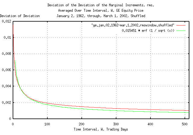
|
Figure XIV is a plot of the cumulative probability of the duration
of the increases and decreases in the deviation of the shuffled
marginal increments, rms, of GE's equity
price with the theoretical value, 0.015451 * erf (1 /
sqrt (t)). The frequency of the durations of the
increases and decreases of up to 506 trading days, (about two calendar
years,) are shown.
|
As a side bar, many quantitative analyst-sometimes called financial engineers-place more importance on the deviation of the marginal increments of time series than any other variable; including asset appreciation. The deviation is a metric of risk. Peter Lynch is accredited with the proverb "making money on Wall Street is easy-keeping it is the hard part." A very small chance of something happening, given enough time, will happen, and that's why its hard. Mitigating risk is how one keeps the money. But we have just seen how difficult it is to get accurate
metrics on risk. Most market technicians use a set of
cross-checks on the metrics of risk. For example, there were
10,113 trading days represented in the time series for GE's
equity price, between January 2, 1962, and March 1, 2002. That
means that the largest daily movement would be a
Its an important concept since statistical anomalies, i.e., those measurements that do not fit a dogmatic model, are often simply discarded in the pseudo-sciences. But what our cross-check is telling us is that our risk of extreme movements in GE's equity price is about 3 times what we think it is! Continuing on, there should be 27 out of 10,000
For 2 sigma events, there should be 460 out of 10,000-and the
460'th largest movement was
Our conclusion is that the model seems to hold fairly well for slightly past 2 sigma events-possibly even to 3 sigma-but beyond 3 sigma, and into 4 sigma, we have to increase our risk assessment metric for an investment in GE's equity by at least a factor of 3. In financial engineering, the excess risk of loss do
to the tail events of the distribution is called Expected
Tail Loss, |
Why the discrepancy?
    tsmath -l ge.jan.02.1962-mar.1.2002 | tslsq -o | tsroot -l | \
        tsscalederivative > ge.jan.02.1962-mar.1.2002
    tsinvestsim -n 1000 sim 10113 | tsmath -l | tslsq -o | tsroot -l | \
        tsscalederivative > tsinvestsim.jan.02.1962-mar.1.2002
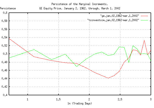
|
Figure XIV is a plot of the persistence in the daily
returns of GE's equity price. Note that there is significant short
term persistence, (about 0.54,) meaning that there is a 54% chance of
GE's equity price doing tomorrow, what it did today. This is probably
a short term inefficiency, (in the sense of the EMH, the Efficient
Market Hypothesis.) However, there is also an indication of a
period of anti-persistence of about e^2.7 =
15 days, too-which is probably related to structural
issues, (for example, a high probability of a cyclic downward
spike every year would do this; probably near late October,
when mutual funds account for capital and income gains for tax
reasons, which can be seen in TABLE I.)
This type of persistence, (actually a cyclic issue,) would increase the likelihood of large swings, and they would tend to cluster. In addition, the leptokurtosis shown in the analysis of GE's equity price in Section I, would tend to increase the relative number of large movements in price.
It would be advantageous to develop a methodology to quantify the persistence/leptokurosis/root inefficiencies of a time series.
In the following analysis, the historical time series of the DJIA,
NASDAQ, and S&P500 indices through December 5, 2002 was obtained
from Yahoo!'s database of equity
Historical Prices, (ticker
symbols ^DJI, ^IXIC, and, ^SPC,
respectively,) in csv format-which was converted to a Unix
database format using the csv2tsinvest
program. The converted filename were
djia1900-2002,
nasdaq1984-2002, and
sp1928-2002, respectively.
    tsmath -l djia1900-2002 | tsroot -l > djia.jan.02.1900-dec.05.2002
    tsmath -l nasdaq1984-2002 | tsroot -l > nasdaq.oct.11.1984-dec.05.2002
    tsmath -l sp1928-2002 | tsroot -l > sp.jan.03.1928-dec.05.2002
    tsinvestsim -n 1000 sim 100000 | tsmath -l | tsroot -l > simulation.100000
where the file sim contains:
dummy, p = 0.51
and is a simulation, for comparison, where the average of the
marginal increments, avg = 0.0004, and
the root-mean-square of the marginal increments, rms =
0.02, giving a likelihood of an up movement,
P, of
0.51-the dynamic characteristics of a
typical equity's value on the US exchanges.
Using the tslsq
to calculate the linear least squares fit approximation of the first
e^3 = 20.0855369232 trading days,
(approximately one calendar month):
    egrep '^[0-2]\.' djia.jan.02.1900-dec.05.2002 | tslsq -p
    -4.915572 + 0.539041t
    egrep '^[0-2]\.' nasdaq.oct.11.1984-dec.05.2002 | tslsq -p
    -4.665253 + 0.558219t
    egrep '^[0-2]\.' sp.jan.03.1928-dec.05.2002 | tslsq -p
    -4.884043 + 0.534678t
    egrep '^[0-2]\.' simulation.100000 | tslsq -p
    -4.138124 + 0.498988t
and plotting for e^4.14709512761 =
63.25 trading days, (about a calendar quarter):
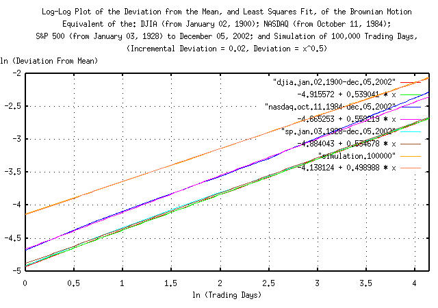
|
Figure XV is a Log-Log plot of the Deviation from the mean, and least squares fit, of the Brownian motion/random walk equivalent of the DJIA, (from January 2, 1900, through, December 5, 2002,) the NASDAQ, (from October 11, 1984, through, December 5, 2002,) the S&P500, (from January 3, 1928, through, December 5, 2002,) and a 100,000 trading day simulation of a typical equity's value from the US exchanges. The slope of the lines in the graph is the root of the deviation-i.e., for the simulation, it would be 0.5, (meaning square root,) or root mean square mathematics should be used, (implying infinite entropy, uncertainty, or unpredictability.)
Of interest is the linearity of the empirical metrics-at least for a calendar quarter of daily closes.
Considering only the dynamics, the deviation of the indices' Brownian motion/random walk equivalent for the DJIA, NASDAQ, and S&P500 from their mean values would be:
    (e^-4.915572) * (t^0.539041) = 0.00733152306 * t^0.539041
    (e^-4.665253) * (t^0.558219) = 0.00941686546 * t^0.558219
    (e^-4.884043) * (t^0.534678) = 0.00756636131 * t^0.534678
respectively, compared with the values derived using the
tsfraction
and tsrms
programs:
    0.011028 * t^0.5
    0.014448 * t^0.5
    0.011367 * t^0.5
respectively. (Note that the exponents represent a system with a Hausdorff
fractal dimension following a power law relationship-for a
Gaussian/normal distribution of the marginal increments, the
relationship is 1 / 0.5 = 2; larger than
0.5 represents a time series with
marginal increments that have a deviation that is non-stable, or
diverging-a Pareto-Levy
distribution-which does have implications; see: Lessons
of the Fall: A Stunning Collapse and Weighty Morals to the
Story.)
And, how much difference is there between the actual, empirical theoretic, and standard deviation approximation for the DJIA, NASDAQ, and S&P500? As an informal, (the deviation is not stable, and diverges,) pictographic interpretation:
    tsmath -l djia1900-2002 | tsroot > djia.jan.02.1900-dec.05.2002.a
    tsmath -l nasdaq1984-2002 | tsroot > nasdaq.oct.11.1984-dec.05.2002.a
    tsmath -l sp1928-2002 | tsroot > sp.jan.03.1928-dec.05.2002.a
and plotting:
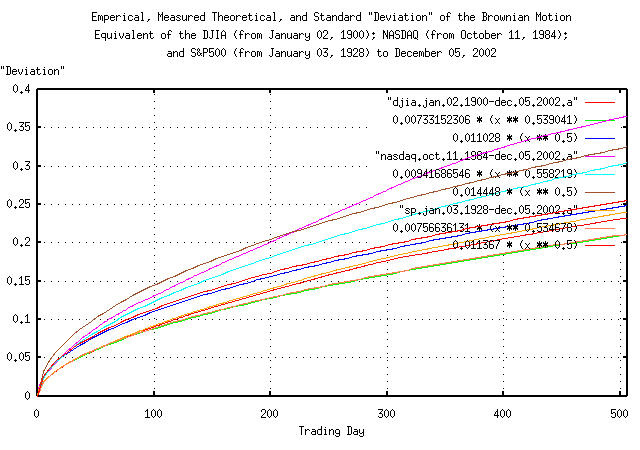
|
Figure XVI is a plot of the "deviation" from the mean, least squares fit of variables, and standard deviation approximation of the Brownian motion/random walk equivalent of the DJIA, (from January 2, 1900, through, December 5, 2002,) the NASDAQ, (from October 11, 1984, through, December 5, 2002,) the S&P500, (from January 3, 1928, through, December 5, 2002,) for 512 trading days, (about two calendar years.) The top three graphs are the NASDAQ, and the DJIA and S&P500 are the bottom six, or approximately a +/- 10% error at two calendar years.
Remember, as a mathematical expediency, the analysis uses the Brownian motion/random walk equivalent of the time series for the indices-to convert back to a log-normal distribution, find the median values, and multiply the median values by the exponentiated values in Figure XVI.
--

John Conover, john@email.johncon.com, http://www.johncon.com/