|
From: John Conover <john@email.johncon.com>
Subject: Quantitative Analysis of Non-Linear High Entropy Economic Systems II
Date: 14 Feb 2002 07:38:46 -0000
As mentioned in Section I, much of applied economics has to address non-linear high entropy systems-those systems characterized by random fluctuations over time-such as net wealth, equity prices, gross domestic product, industrial markets, etc.
The characteristic frequency distributions, over time, of non-linear high entropy systems evolve into log-normal distributions requiring suitable methodologies for analysis.
Note: the C source code to all programs used are available from the NtropiX Utilities page, or, the NdustriX Utilities page, and are distributed under License.
|
|
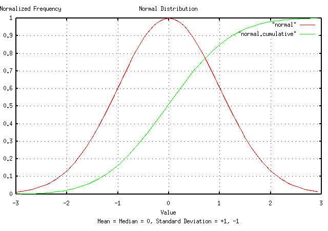
Figure I presents a normal/Gaussian frequency distribution made
with the tsgaussian,
and, tsnormal
programs. The distribution was integrated, using the tsintegrate
program, and the X-Axis values modified using the tsmath
program such that both the distribution and its cumulative fit on the
plot. The root-mean-square, (i.e., the deviation,) of the distribution
is unity, and the mean equals the median, which is zero.
If the difference of the increments of a system are
characterized by a normal/Gaussian distribution-i.e., Brownian
motion, or a random walk-then the system is a cumulative
sum of a random variable, a(t), with a
normal/Gaussian distribution; an additive construct:
V(n + 1) = V(n) + a(t) .............................(2.1)
However, the non-linear, high entropy economic model described in
Section
I, is a multiplicative construct-it is a geometric
progression of a random variable,
a(t), with a normal/Gaussian
distribution:
V(n + 1) = V(n) * (1 + a(t)) .......................(2.2)
which has a long term evolutionary distribution that is log-normal, (although the marginal increments have a normal/Gaussian distribution.)
To make a log-normal distribution from a normal/Gaussian
distribution, the X-Axis is exponentiated, (i.e., for each
number on the X-Axis, use e to that
number, to make a new X-Axis for a log-normal plot.)
|
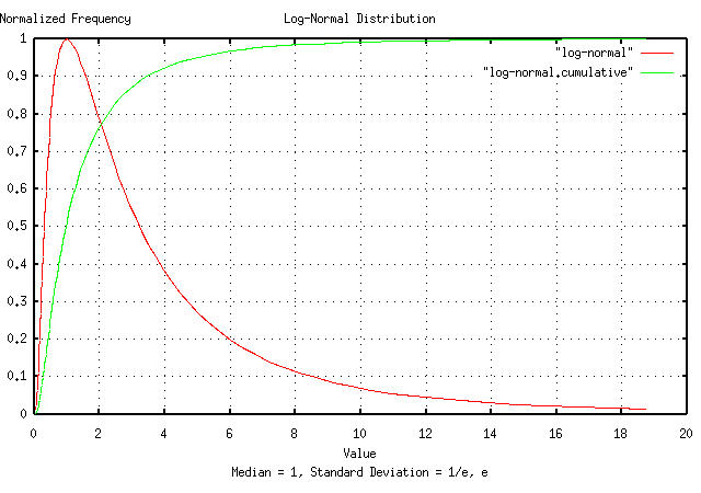
Figure II is a plot of the normal/Gaussian frequency distribution,
shown in Figure I, and its cumulative, with the X-Axis exponentiated,
using the tsmath
program. Note that the mean
diverges to infinity, (i.e., becomes undefined,) for the log-normal
distribution. The median of the log-normal distribution,
medianLN is:
                meanN
    medianLN = e      ..................................(2.3)
where meanN is the mean of the
normal/Gaussian distribution. The one
deviation values, sdLN+, and
sdLN-, of the log-normal distribution
are:
             sdN
    sdLN+ = e    * medianLN ............................(2.4)
             -sdN
    sdLN- = e     * medianLN ...........................(2.5)
where sdN is the deviation of the
normal/Gaussian distribution, and sdLN+
is the high side deviation for the log-normal distribution, and
sdLN-, the lower side. Likewise, the two
deviation values for the log-normal distribution are
e^2sdN * medianLN and
e^-2sdN * medianLN, and so on.
The term deviation in normal/Gaussian and log-normal distributions has the same meaning; for the cumulative, 84.1344746068542954% of the time, the value will be less than one deviation, 97.7249868051820868% of the time less than two deviations, and so on.
As a methodology, we can map back and fourth between log-normal and normal/Gaussian distributions. To convert a log-normal frequency distribution to a normal/Gaussian distribution, take the log of the X-Axis. To convert back to a log-normal distribution, exponentiate the X-Axis. The median of the log-normal distribution is the mean of the normal/Gaussian distribution, exponentiated. The deviation values of the log-normal distribution are the median of the log-normal distribution, multiplied by by both plus and minus the deviation of the normal/Gaussian distribution, exponentiated.
|
As a side bar, it is frequently expedient-particularly when
analyzing the dynamics of a high entropy non-linear system with
log-normal characteristics-to work with the Brownian
motion/random walk equivalent of the system's time series. The
system's time series can be converted back and forth between the
two, for example, (using the time series,
and: will convert a DJIA time series to its Brownian motion/random walk equivalent, and back. Different techniques are offered in Appendix I. |
The relationship between the median of the log-normal distribution,
medianLN, and the median of the Brownian
motion/random walk equivalent, meanN,
is:
                meanN
    medianLN = e      ..................................(2.3)
The relationship between the one deviation value of the Brownian
motion/random walk equivilent, sdN, and
the one deviation values, sdLN+, and
sdLN-, of the log-normal distribution
are:
             sdN
    sdLN+ = e    * medianLN ............................(2.4)
and:
             -sdN
    sdLN- = e     * medianLN ...........................(2.5)
respectively.
Suppose a high entropy economic system has daily marginal
increments with a root-mean-square value of the deviation equal to
0.02, (i.e., 2% per day, which would be a typical value for
an equity price on the US markets, the US GDP, or an industrial market
growth/market share, etc.) At the end of a calendar year, consisting
of 253 business days, the estimate, (using the Brownian motion/random
walk model-as applied in classic Black-Scholes-Merton
methodology,) for the root-mean-square of the frequency distribution
of system's value, (i.e., the equity's increase in value after
investing a calendar year,) would be 0.02 * sqrt (253) =
0.318119474; meaning that for 84.1344746068542954% of
the time, an annual investment would increase in value by less than
31.8119474%, (and 50% of the time, the investment would decrease in
value.)
|
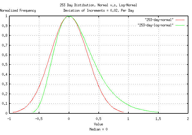
Figure III is a plot of the normal/Gaussian frequency distribution
of the investment's value at the end of a calendar year using a random
walk model, and the non-linear high entropy model described in Section
I which produces a log-normal distribution. The graphs were
shifted using the tsmath
program for comparison of the two distributions' deviations from their
median values.
For the log-normal distribution, the deviations are
e^0.318119474 = 1.37454047383, or a high
side deviation of 37.454047383%, and e^-0.318119474 =
0.727515864, or a low side deviation of 27.2484136%,
compared with the random walk model's deviations of +31.8119474%, and
-31.8119474%; an accuracy within 10% for for one deviation.
However, if we extrapolate the random walk model's deviation to three deviations, (i.e., 3 * 0.318119474 = 0.95435842149,) and expect the investment's value to be less than that for 99.8650101968363646% of the time, we have committed a two order of magnitude error in the assessment of risk! (Restated approximately-instead of the investment's gain in value being lower than a factor of 2 in one calendar year, 0.1% of the time, its actually, 10% of the time.)
The median household net wealth in the US is about $40,000 from http://www.whitehouse.gov/fsbr/income.html, and there are about a hundred million households in the US. Bill Gates' family is the richest in the US, with an estimated net wealth of around fifty billion dollars. What are the chances that any household, in the 25 year period that it took Gates to acquire his wealth, could have become the richest in the US, using a typical value for the daily variance of wealth of 3%?
Assuming wealth distribution in a society is log-normal, and using
the methodology outlined above, on the normal/Gaussian distribution's
X-Axis scale, the log-normal median would become the mean,
ln (40000) = 10.5966347331, and Gates'
net wealth would be ln (50000000000) =
24.6352888424. The deviation of the normal/Gaussian
distribution would be 0.03 * sqrt (25 * 253) =
2.38589605809 after 25 years of 253 business days.
We now have to solve the equation n = (24.6352888424
- 10.5966347331) / 2.38589605809, where
n is the number of deviations that
separate the Gates' family from the mean in the normal/Gaussian
distribution, or n = 5.88401747918
deviations.
But we already knew that answer. What number of deviations is one
household in one hundred million?
5.616.
With a US median wealth of about $40,000, in any 25 year period, it is a virtual certainty that one person will have a net worth in the many billions of dollars. Whether Bill Gates won the lottery of the non-linear high entropy economic system to get the tail point in the log-normal distribution, or is a genius depends on who is telling the story.
Of passing interest, the distribution of a country's wealth is characterized by the median, and not the arithmetic average; the calculation of the average is not stable, and diverges to infinity in the evolution of log-normal distributions-the term average wealth of a country makes no sense. The peak of the log-normal bell curve lies below the median, also-meaning that the largest frequency of wealth is below the median value.
In other words, without wealth re-distribution, a society's household wealth will evolve into a log-normal distribution; the rich get richer, and the poor get poorer-relative to the rich-with an ever widening gap between the two.
|
As a side bar, it would seem-at least intuitively-that the the rich provide the capital which fuels the expansion of the economy. But in general, that is not necessarily the case. To illustrate the point, consider a very simple economy,
where the participants increase wealth, through productivity, at
about and from Section I, Equation (1.20), for each household, without taxation or wealth re-distribution. Now, consider there is a benevolent king that goes around to every household in the simple society, every day, and collects 100% of the household's earnings for the day, then redistributes the society's total earnings, equally, to each household, (e.g., a 100% taxation rate and re-distribution,) which the households can do with, as they wish. Then, Equation (1.24) from Section I becomes: since the standard deviation,
And, Equation (1.20) from Section I becomes: doubling the society's GDP expansion. Note that all industrialized countries have progressive
tax systems-which approximate both cases of the simple
society, above, (the numbers used, Now, consider that the king of the simple society is not so benevolent, and has his fingers in the till, (representing corruption, pork, or other wasteful spending that does not enhance the future welfare of the society as a whole.) If the king steals more than 0.02% per day, the simple society is doomed-its economy will deteriorate into nothing. The moral? Increasing tax rates is not necessarily detrimental to the growth of the GDP-and can even enhance it-provided the government is efficient, (and an efficient government is more important than the tax rate in determining the increase in prosperity, over time.) |
According to the March, 1999 article in Information Today, Microsoft had an 86 percent marketshare of the desktop computer market, and Linux, 2.5 percent. What are the chances of Linux becoming dominant in the desktop marketplace?
We can use the Brownian motion/random walk equivalent of the
non-linear high entropy desktop marketplace, and treat the problem as
a gambler's
ruin; ln (0.82) = -0.198450939, and
ln (0.025) = -3.68887945411, and the
probability, L, of Linux supplanting
Microsoft would be:
         -0.198450939
    L = -------------- = 0.0537970788
        -3.68887945411
or, about 5%, or about one in twenty.
Technically, the few percentage point chance is the chance that Microsoft will fall out of favor, (or go bust,) before Linux does-like the gambler's ruin, the chance of the house going broke before the player does is virtually zero-even if the game is fair.
But that does not mean Microsoft is invincible-it would take 20 attempts to cut Microsoft's chances of remaining on top to 50%. And how many attempts has their been? Corel, FreeBSD, Sun, Linux, Borland, Apple, Digital Research, DEC, SCO, UnixWare, AT&T, IBM OS/2, AIX, etc., all of which have/had a few percentage points of the desktop marketshare.
|
As a side bar, for the initiated, the technique used here is not inconsistent with Cournot-Nash equilibrium for the duopoly. It does assume, as a first order approximation, that the equilibrium has simple fractal characteristics. Interestingly, Cournot-Nash equilibrium is similar to the iterated prisoner's dilemma strategic game; probably the simplest of all games where the players have to make decisions under uncertainty do to conflict of interest and self-referentiality, which is why the characteristics are stochastic in nature. The concept of self-referential indeterminacy is ubiquitous in modern economics. It would be difficult to underestimate the contributions of the penetrating intellects of Gérard Debreu and Kenneth Arrow to modern economics. Note that Walrasian General Equilibrium Theory, the static equilibrium concepts popularized by Marshall and Keynes, is qualitatively different than Cournot-Nash equilibrium. The concept of static general equilibrium was dealt a fatal intellectual blow by Debreu Sonnenschein and Mantel, (DSM,) in the early 1970's, and has largely been discounted. |
We could, also, approximate the non-linear high entropy marketplace of the computer desktop with a Brownian motion fractal, in which case, the gambler's ruin becomes:
        0.025
    L = ----- = 0.0304878049
        0.82
or, about 3%, or about 1 in 33, which is a reasonably good approximation for such small probabilities.
It is often expedient to convert a time series with log-normal characteristics, (for example, equity prices and index values, industrial market metrics, and GDPs,) to a Brownian motion/random walk equivalent-which is the simplest fractal, and has a large mathematical infrastructure dating back to the Sixteenth Century.
To explore the different techniques available for converting a time
series with log-normal characteristics to its Brownian motion/random
walk equivalent, the tsinvestsim
program will be used to generate a time series with known log-normal
characteristics, and the simulation converted to its Brownian
motion/random walk equivalent using the different techniques. The
characteristics are defined in a single file,
ts, which contains the single
record, "dummy, p = 0.51".
The log-normal characteristics of the simulation will have an
average and deviation of the marginal increments, avg =
0.0004 and rms = 0.02,
respectively, a marginal gain, g =
1.0002, and a likelihood of an up movement,
P = 0.51, using Equation
(1.24), and, Equation
(1.20). The time series will have 100,000 time units. (For an
example of such a simulation, see the analysis of GE
Equity Price in Section
I.)
The simplest two ways of conversion:
    tsinvestsim -n 1000 ts 100000 | tsmath -l > tsinvestsim.tsmath-l
    tsinvestsim -n 1000 ts 100000 | tsfraction | \
        tsintegrate > tsinvestsim.tsfraction.tsintegrate
And plotting:
|
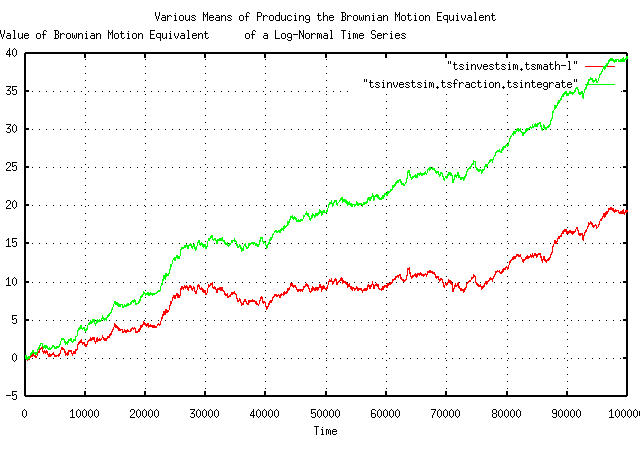
Figure IV is a plot of the Brownian motion/random walk equivalent
of the simulated time series. The first technique just takes the
natural logarithm, using the tsmath
program, of each element in the time series-since a geometric
progression of a random variable has exponential characteristics,
taking the logarithm linearizes the time series. The second
technique finds the marginal increments of each element, using the
tsfraction
program, which is the random sequence of fluctuations in the simulated
time series, and integrates it using the tsintegrate
program-a Brownian motion/random walk is always the cumulative sum, or
integration, of a random process.
Note that the two graphs in Figure I are identical, except in
slope. The slope of the top line is avg =
0.0004, (note that this is a technique for measuring
avg,) and the slope of the bottom line
is ln (g) = ln (1.0002) ~ 0.0002, (which
is a technique for measuring, g, too.)
Of passing interest is that the gain, g,
is not the average, avg, of the marginal
increments of the time series of a non-linear high entropy system with
log-normal characteristics, (a subtle fact that has bitten
many using regression analysis.)
Of interest is the straight line slope; in the case of taking the natural logarithm of each element in the time series, it represents the median value of the log-normally distributed time series. If the value of the Brownian motion/random walk equivalent is above this line, it is a positive bubble-likewise, if it is below the line, it is a negative bubble. The distance the value is away from the straight line slope is the magnitude of the bubble, and the time between crossings of the straight line slope, the duration of the bubble. Fortunately, there is a large mathematical infrastructure for analyzing Brownian motion/random walk bubbles, (which will be explored in Section III, and, Section IV.)
When analyzing the dynamics of non-linear high entropy economic
systems, i.e., the duration and magnitude of bubbles, it is
frequently advantageous to eliminate the slope in the conversion to a
Brownian motion/random walk equivalent fractal. There are two common
methods: subtract the average, avg, from
the marginal increments of the time series; least squares fit the
slope of the Brownian motion/random walk equivalent. The first
subtracts a slope that is calculated using the average of the
marginal increments, the latter subtracts a slope that is calculated
using the variance of the marginal increments. If the data
set size is sufficient, both will produce nearly identical
results.
There is a third method of removing the slope in the conversion of
a non-linear high entropy system's log-normal characteristics to a
Brownian motion/random walk equivalent, and that is to subtract a
value that will make the gain, g,
unity.
From Section I:
        avg
        --- + 1
        rms
    P = ------- ........................................(1.24)
           2
or:
                avg
            1 - ---
                rms
    1 - P = ------- ....................................(2.6)
               2
and substituting into:
                 P          (1 - P)
    g = (1 + rms)  (1 - rms)        ....................(1.20)
after taking the natural logarithm of each side:
                      avg
    2 * ln (g) = (1 + ---) * ln (1 + rms) +
                      rms

                      avg
                 (1 - ---) * ln (1 - rms) ..............(2.7)
                      rms
and manipulating for avg:
                                avg
    2 * ln (g) = ln (1 + rms) + --- * ln (1 + rms) +
                                rms

                 ln (1 - rms) -

                 avg
                 --- * ln (1 - rms) ....................(2.8)
                 rms
or:
    avg                  avg
    --- * ln (1 + rms) - --- * ln (1 - rms) =
    rms                  rms

        2 * ln (g) - ln (1 + rms) - ln (1 - rms) .......(2.9)
and if g = 1, then:
    avg * ln (1 + rms) - avg * ln (1 - rms) =

        rms (- ln (1 + rms) - ln (1 - rms)) ............(2.10)
and, finally:
          rms (- ln (1 + rms) - ln (1 - rms))
    avg = ----------------------------------- ..........(2.11)
              ln (1 + rms) - ln (1 - rms)
for g = 1.
Of passing interest, making avg = 0
will not make g = 1; it will
make it negative.
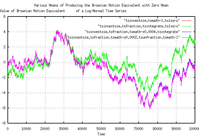
So, there are several techniques available to remove the straight line slope in the conversion from a non-linear log-normal time series to a Brownian motion/random walk equivalent:
    tsinvestsim -n 1000 ts 100000 | tsmath -l | tslsq -o > tsinvestsim.tsmath-l.tslsq-o
    tsinvestsim -n 1000 ts 100000 | tsfraction | tsintegrate | \
        tslsq -o > tsinvestsim.tsfraction.tsintegrate.tslsq-o
    tsinvestsim -n 1000 ts 100000 | tsfraction | tsmath -s 0.0004 | \
        tsintegrate > tsinvestsim.tsfraction.tsmath-s0.0004.tsintegrate
    tsinvestsim -n 1000 ts 100000 | tsfraction | tsmath -s 0.0002 | tsunfraction | \
        tsmath -l > tsinvestsim.tsfraction.tsmath-s0.0002.tsunfraction.tsmath-l
And plotting:
|
Figure V is a plot of the detrended, (i.e., with the
straight line slope removed,) Brownian motion/random walk equivalent
of the simulated non-linear log-normal time series. The first two
techniques just use the tslsq
program to least squares fit, and subtract, the slope of the lines in
Figure IV. The third technique subtracts the average,
avg of the marginal increments, using
tsfraction
and the tsmath
programs, and integrates, using the tsintegrate,
program to produce the Brownian motion/random walk equivalent. The
forth technique uses Equation
(2.11), and is similar to the third techique, but uses the
tsunfraction
program to construct the Brownian motion/random walk equivalent.
Which technique should be used? Probably:
tsmath -l ts | tslsq -o > ts.brownian.zero.mean
is probably the easiest, and most reliable. But many will use one
of the averaging and least
squares techniques, both-in general, they converge
from opposite directions, and it is a handy thing to know if there is
a convergence problem, (like the data set size is too small.)
Note that the Y-Axis values in Figures IV and V are the Brownian motion/random walk equivalents. To convert back to non-linear log-normal characteristics, (using the previous example):
tsmath -l ts | tslsq -o | tsmath -e > ts.log-normal.unity.median
which will give the minimum variance, exponentially detrended, non-linear log-normal characteristics of the time series with a median of unity-and is a very useful technique.
--

John Conover, john@email.johncon.com, http://www.johncon.com/