|
From: John Conover <john@email.johncon.com>
Subject: Quantitative Analysis of Non-Linear High Entropy Economic Systems Addendum
Date: 14 Feb 2002 07:38:46 -0000
As mentioned in Section I, Section II, Section III, Section IV, Section V and Section VI, much of applied economics has to address non-linear high entropy systems-those systems characterized by random fluctuations over time-such as net wealth, equity prices, gross domestic product, industrial markets, etc.
Do to the interest generated, the US GDP will be revisited, the NASDAQ index analyzed, and a comparison of the DJIA, NASDAQ, and S&P500 declines offered, using up-to-date data. Appendix II concludes with an analysis of the significant declines in the US equity market indices over the last hundred years-and offers a simple methodology for calculating the severity of the declines.
Note: the C source code to all programs used is available from the NtropiX Utilities page, or, the NdustriX Utilities page, and is distributed under License.
The historical time series of the US GDP, from 1947Q1 through 2002Q1, inclusive, was obtained from http://www.bea.doc.gov/bea/dn/nipaweb/DownSS2.asp, file Section1All_csv.csv, and Table 1.2. Real Gross Domestic Product Billions of chained (1996) dollars; seasonally adjusted at annual rates, manipulated in a text editor to produce the US GDP time series data.
|
|
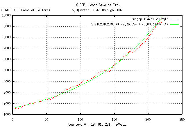
Figure I is a plot of US GDP data. The formula for the least
squares fit to the data was determined by using the tslsq
program with the -e -p options. The
least squares fit is the median value of the US GDP. From 1947 through
2002, the US GDP expanded at 0.8339% per
quarter, or a 1.008339^4 = 1.0337755579 =
3.37755579% annual rate.
|
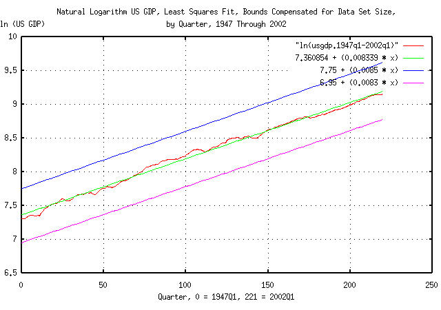
Figure II is a plot of the Brownian motion/random walk fractal
equivalent of the US GDP, as described in Section
II, using the data in Figure I. The data for Figure II was
constructed using the tsmath
program with the -l option. The least
squares fit of the data was determined by using the tslsq
program with the -p option. The least
squares fit of the data is the median value of the Brownian
motion/random walk fractal equivalent of the US GDP. The average,
avg, and deviation,
rms, of the marginal increments of the
US GDP were determined by using the tsfraction
program on the data in Figure I, and piping the output to the
tsavg
and tsrms
programs using the -p option,
respectively. The average, avg, and
deviation, rms, of the marginal
increments of the US GDP were used as arguments for the
tsshannoneffective
for calculating the range of uncertainty do to the limited data set
size of 221 elements in the time
series. The actual median value of the Brownian motion/random walk
fractal equivalent of the US GDP is a straight line that is bounded by
the upper and lower limits shown in Figure II. The line does not have
to be parallel to these limits.
|
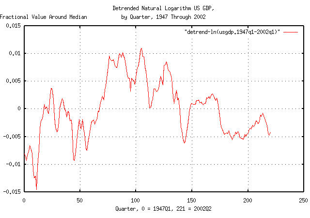
Figure III is a plot of the data in Figure II after using the
tslsq
program with the -o option to remove the
linear trend in the median value of the Brownian motion/random walk
fractal equivalent of the US GDP. The Figure represents how far the
actual Brownian motion/random walk fractal equivalent of the US GDP is
from its median value. For example, at Q1, 1967, (80 quarters past Q1,
1947,) the Brownian motion/random walk fractal equivalent of the US
GDP was about 1% above its median value.
|
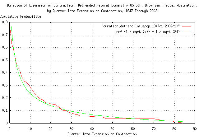
Figure IV is a plot of the distribution of the cumulative run
lengths, (durations,) of the expansions and contractions in the
Brownian motion/random walk fractal equivalent of the US GDP. It was
constructed using the tsrunlength
program on the data in Figure III. The theoretical Brownian
motion/random walk fractal abstraction for the data is shown for
comparison. The longest run length in the data was 84 quarters do to
limited data set size. As an approximation, the theoretical data was
offset by erf (1 / sqrt (84)), which is
about 1 / sqrt (t) for t
>> 1. The distribution of the expansions and
contractions is applicable to the log-normally distributed durations
in Figure I. For example, the chances of a contraction, or expansion,
of ten quarters continuing at least through the eleventh is about 25%,
where expansion and contraction is defined as being above, or below,
the median value shown in Figure I or Figure II.
|
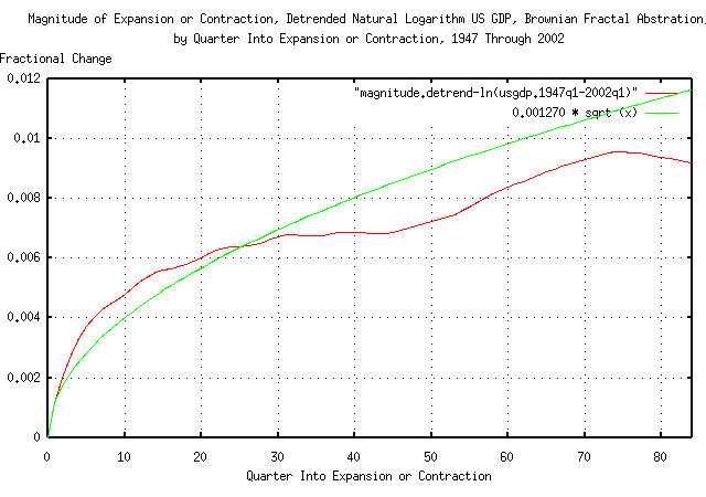
Figure V is a plot of the magnitude of the deviations of the
expansions and contractions in the Brownian motion/random walk fractal
equivalent of the US GDP. It was constructed using the
tsrunmagnitude
program on the data in Figure III. The theoretical Brownian
motion/random walk fractal abstraction for the data is shown for
comparison, which was calculated by using the tsderivative
program on the data in Figure III, and piping the output to the
tsrms
program with the -p option. The
deviation of the marginal increments of the data in Figure III is
0.001270. For example, the deviation
from the median value of the Brownian motion/random walk fractal
equivalent of the US GDP at 70 quarters
would be a little more than 1% from its
median value, i.e., for about 68% of the time, at 70 quarters, the
value of the Brownian motion/random walk fractal equivalent of the US
GDP would be within about +/- 1% from
its median value. This is not applicable to the log-normally
distributed expansions and contractions in Figure I.
|
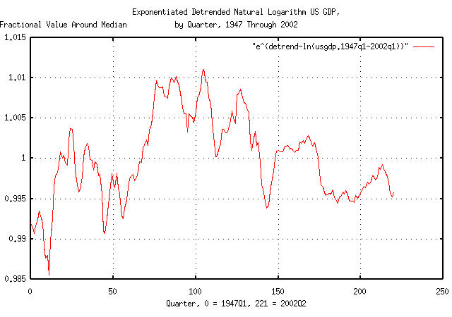
Figure VI is a plot of the data in Figure III exponentiated by
using the tsmath
program with the -e option. This is the
graph of the dynamics of the US GDP as shown in Figure I. An example
interpretation of Figure VI, at Q1, 1967, (80 quarters past Q1, 1947,)
is that the US GDP was about 1% higher than its median value, i.e.,
multiply the median value at 8 quarters by 1.01.
|
As a side bar, the relationship between Figure VI and Figure
III is interesting. As an approximation to the US GDP, Black-Scholes-Merton,
methodology can be used since the data in the two graphs is
essentially the same-differing only by a constant of unity. The
reason is that |
To reiterate what was done, the US GDP data, in Figure I, was
converted to its Brownian motion/random walk fractal equivalent as
shown in Figure II. This data was linearly detrended in Figure III,
and the distribution of the run lengths, (durations,) and magnitude of
the expansions and contractions compared against the theoretical
abstraction of a Brownian motion/random walk fractal, as shown in
Figure IV and Figure V, (to gain confidence in the fractal assumptions
about the data.) The linearly detrended data in Figure III was then
exponentiated, as shown in Figure VI, and illustrates the dynamics of
the US GDP data in Figure I. (Additionally, as a cross-check, the
consecutive like movements in the marginal increments of the data in
Figure VI was counted by hand and assembled into a distribution
histogram-the distribution was found to be reasonably close to the
theoretical 0.5 / n distribution.)
Note from Figure VI that the US GDP has been in a chronic mild
recession since the end of Q1, 1990, (174 quarters past Q1, 1947,) or,
for about 47 quarters. Its performance has been below its median
value, despite the economic bubble of the late 1990's. From
Figure IV, the chances of the mild recession continuing is about
1 / sqrt (47) = 0.145864991 = 14.6%, or
the chances of it ending soon is about
85.4%. It would be anticipated that the
US GDP expansion would be increased by about 1-1.5% from where it was
in the 1990's, (or now,) with a 50% chance of it lasting at least 5
quarters, (because erf (1 / sqrt (4.396233)) = 0.5 =
50%.) The optimal fraction-at-risk for such a scenario
would be 2 * 0.854 - 1 = 0.708 = 70.8%,
i.e., place 71% at risk to exploit the
opportunity of a 5 quarter expansion of 1% in the US GDP, while
holding 29% in reserve.
With like reasoning, the current relative economic recession,
(relative to the bubble of the late 1990's-the only way we
can analyze it when it is contained in the chronic mild recession
analyzed above; the recession started below the median value of the
GDP,) which started at the end of Q2, 2000, (214 quarters past Q1,
1947,) or, seven quarters ago, has a chance of continuing of about
1 / sqrt (7) = 0.37796447301 = 37.8%,
meaning that the chances of the current relative economic recession
returning soon to its value of 8 quarters ago would be about
62.2%. The optimal fraction-at-risk for
such a scenario would be 2 * 0.622 - 1 = 0.244 =
24.4%, i.e., place 24%
at risk to exploit the opportunity of the GDP returning to its value
in Q1, 2000, while holding 76% in
reserve.
All-in-all, late 2002 seems to be an opportunistic time to start a company-with a minimal risk, (about 30% at that time,) of having to drag the GDP uphill, (probably on a par with 1984 and 1995.)
The historical time series of the NASDAQ index, from October 11,
1984 through May 3, 2002, inclusive, was obtained from Yahoo!'s database of equity Historical Prices, (ticker symbol
^IXIC,) in csv format. The csv format was
converted to a Unix database format using the csv2tsinvest
program.
|
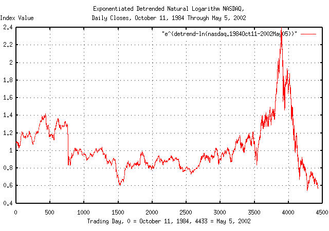
Figure VII is a plot of the exponentiated, detrended, natural
logarithm of the NASDAQ index Unix database file,
nasdaq1984-2002. It was made
with the single piped command:
tsmath -l nasdaq1984-2002 | tslsq -o | tsmath -e > 'e^(detrend-ln(nasdaq.1984Oct11-2002May05))'
This is the graph of the dynamics of the NASDAQ index. An example interpretation of Figure VII, at March 10, 2000, (3,895 trading days past October 11, 1984,) is that the NASDAQ index was about 2.4 times its median value, i.e., multiply the median value at 3,895 trading days by 2.4.
|
As a side bar, it is rather obvious from Figure VII why the NASDAQ fell so hard; on March 10, 2000, the NASDAQ index was over valued by a factor of 2.4. The NASDAQ was in a speculative bubble. The median value of the NASDAQ is its average fair market value, (by definition-half the time the value will be more, half less.) That the NASDAQ was in a speculative bubble was apparent by late 1999, (around trading day 3,750 past October 11, 1984.) Speculative bubbles that inflate values by factors of 2, (even orders of magnitude,) in high entropy economic systems are not uncommon, at all. If there is a new economy, its valuations are still subject to to the hazards of speculation-just like the old one. |
Note from Figure VII that the current deflation in the NASDAQ's
value started on February 16, 2001, (4,132 trading days past October
11, 1984,) when it dropped below its median value, 2425.38. That's
when the NASDAQ became under valued. On an annual basis, it would be
expected that there is a 50% chance that the NASDAQ remain under
valued for less than 4.396233 years, (erf (1 / sqrt
(4.396233)) = 0.5,) and a 50% chance that it
wouldn't. So, there is a 50% chance that on July 6, 2005, its value
will be back above its median value, which on that date would be
3895.04.
Also, there is a 50% chance that the NASDAQ will bottom before about half the 4.396233 years, (i.e., by about April 29, 2003,) and a 50% chance after. When it bottoms, there is a 15.87% chance, (i.e., one standard deviation,) that the NASDAQ index value would be below 2209.76, (and a 15.87% chance that it would be above than 4275.11.) Its median value on April 29, 2003 would be 3073.59.
Or, the chance, (where the chance is approximately 1
- 1 / sqrt (t),) that the bottom of the decline will
occur by a specific month:
|
As a side bar, November, 2004 is the month of the
Presidential election in the US, and there is a 45% chance that
the equity market performance will be an issue, and a 55% that
it won't-whoever wins will have a good chance to claim credit
for a 4.4 year-median duration-increasingly prosperous equity
market. The optimal political strategy is to place a
|
All-in-all, early to mid 2003 seems to be an opportunistic time to start a technology company-with a minimal risk of having to drag the equity market uphill, (probably on a par with 1984 and 1995.)
The historical time series of the DJIA, NASDAQ, and S&P500
indices through July 26, 2002 was obtained from Yahoo!'s database of equity Historical Prices, (ticker
symbols ^DJI, ^IXIC, and, ^SPC,
respectively,) in csv format. The csv format was
converted to a Unix database format using the csv2tsinvest
program. (The DJIA time series started at January 2, 1900, the NASDAQ
at October 11, 1984, and January 3, 1928 for the S&P500.)
The deviation, rms, of the marginal
increments of the indices was determined by using the tsfraction
program and piping the output to the tsrms
program using the -p option. The
deviation of the marginal increments of the DJIA was 0.010988,
0.014191 for the NASDAQ, and 0.011313 for the S&P500.
The daily fractional gain for each of the indices was found using
the tsgain
program with the -p option, and found to be 1.000171 for the DJIA,
1.000366 for the NASDAQ, and 1.000196 for the S&P500.
The maximum value of each of the indices was found using the
tsmath
program with the -M option, and found to be 11723.00 for the DJIA on
January 14, 2000; 5048.62 for the NASDAQ on March 10, 2000, and,
1527.46 for the S&500 on March 23, 2000.
Since the DJIA was the first to decline, the time series file for
each of indices was trimmed, using the Unix tail(1) command, to the
last 631 trading days-meaning each file starts on January 14, 2000,
and ends on July 26, 2002. Each of these files were, point by point,
divided by its the maximum value, using the tsmath
program with the -d option, such that the maximum in each of the
indices was unity, and the graphs plotted.
|
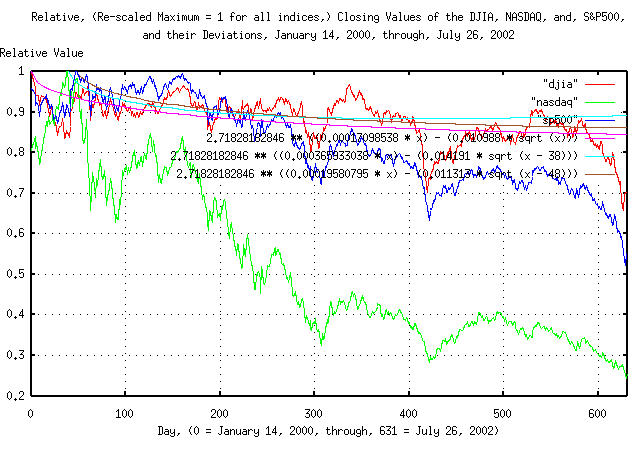
Figure VIII is a plot of the re-scaled DJIA, NASDAQ, and S&P500
indices, from January 14, 2000, through July 26, 2002. The maximum
value in each of the indices was re-scaled to unity. The deviation of
the indices are also shown; 2.71828182846 **
((0.00017098538 * x) - (0.010988 * sqrt (x))) for the
DJIA, 2.71828182846 ** ((0.000365933038 * x) - (0.014191
* sqrt (x - 38))) for the NASDAQ, and,
2.71828182846 ** ((0.00019580795 * x) - (0.011313 * sqrt
(x - 48)))
for the S&500, (the values
0.00017098538,
0.000365933038, and,
0.00019580795, are the natural logarithm
of the gain values, above, 1.000171, 1.000366, and, 1.000196,
respectively-it is important to remember that the graphs of the
indices in Figure VIII are a modeled as geometric sequence, and have a
log-normal distribution; see Section
II, for particulars.
The interpretation of Figure VIII is that the value of an Index will be below its deviation for one standard deviation of the time, (i.e., it will be below the deviation line for 15.866% of the time, and above it, 84.134% of the time.) For example, the DJIA, at 200 days into any "bear" market, would have declined more than 10% about 16% of the time.
The final value for the DJIA in Figure VIII was 0.704972, 0.249993 for the NASDAQ, and, 0.558339 for the S&P500.
|
As a side bar, it can be seen that the magnitude of
the decline in the DJIA is not outside the realm of
expectation. (As a sanity check, there were ((253 * 100) - 631) chances in
the Twentieth Century for such things, or we should have seen
(((253 * 100) - 631) / 85), or about 290; a little work with an
sh(1) control loop script using tail(1), and the However, for the S&P500, the magnitude of the
decline is about a And, for the NASDAQ, the magnitude of the decline is
about a But that's not the whole story. The chances, (for all indices,) of a decline, from their median
value, lasting at least 631 days is Additionally, there is a 50%, (e.g., the median value,) chance
of the bottom of the decline occurring before where
|
The astute reader would notice a slight discrepancy with the analysis
of the NASDAQ, earlier, where the values of the variables were
derived by a least-squares best fit technique, (using the
tslsq
program,) instead of the averaged values. Although both methodologies
use Kalman
filtering techniques, both methods will give slightly different
results unless the data set size is adequately large.
It can be shown that Kalman filtering techniques provide the best metric accuracy possible, for a given data set size, when analyzing stochastic systems-but how good is the best?
    tsfraction djia | tsstatest -c 0.84134474607 -e 0.0000368080189
    For a mean of 0.000232, with a confidence level of 0.841345
        that the error did not exceed 0.000037, 177081 samples would be required.
        (With 28047 samples, the estimated error is 0.000092 = 39.899222 percent.)
    For a standard deviation of 0.010988, with a confidence level of 0.841345
        that the error did not exceed 0.000037, 88541 samples would be required.
        (With 28047 samples, the estimated error is 0.000065 = 0.595169 percent.)
says that for the average, avg, of
the marginal increments of the DJIA's time series (assumed to be
0.000232,) to be known to within one standard deviation, with a
confidence of one standard deviation, the DJIA's time series would
have to have 177,081 samples, or about 700 years, (of 253 trading days
per year.) The time series used in the analysis was about one seventh
of that, and the error created by the inadequate data set size is
about 40%. This means, that if this test was run on different, but
statistically similar, data sets of 28,049 samples, the average of the
marginal increments, avg, would fall
between 0.0001392 and 0.0003248, for one standard deviation = 68.269%
of the time, (if it really is 0.000232; but we really don't know
that-that is just what was measured.) See Appendix
I for particulars.
At issue is the average of the marginal increments,
avg, "rattling around" in numbers which
are the deviation of the marginal increments,
rms, which is about 47 times larger for
the DJIA time series. Any competently designed trading software will
accommodate such data set size uncertainties, (hint: the uncertainty
do to data set size is a probability for a range of values and the
decision variable for the quality of an equity is the probability of
an up movement-multiply them together to get the probability of an up
movement, compensated for data set size.)
Its all the more sobering when one considers that the coefficient
of exponentiation in the DJIA's time series is proportional to the
avg!
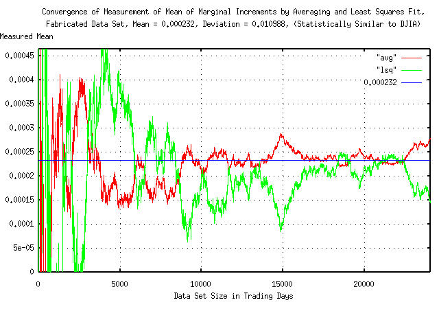
As an example of the convergence of the measurement of the mean of
the marginal increments, avg, of a time
series, a data set was constructed using the tsinvestsim
program, (using the -n 1000 option for 0.1% granularity in the
binomial distribution,) with P =
0.51055697124 and F =
0.010988, which would produce a time series that is
statistically similar to the DJIA time series analyzed in The
relative declines of the DJIA, NASDAQ, and S&P500 Indices, and
the data set size analysis, A
Note About The Accuracy of the Analysis, above. The mean of the
marginal increments, avg, will be
exactly 0.000232, and the deviation,
rms, 0.010988.
The marginal increments of the fabricated time series were produced
by the tsfraction
program, and piped to both the tsavg
and tslsq
programs for comparison of convergence for the first 28048 records of
the time series, using the Unix head(1) command, and the convergence
plotted.
|
Figure IX is a plot of the convergence of the mean of the marginal
increments, avg, by averaging and least
squares fit on the fabricated data set with a mean of exactly 0.000232
and a deviation of 0.010988. The top of the graph is a positive 100%
error, and the bottom, negative 100%-for the first 1000 elements of
the data set, (corresponding to about 4 calendar years,) errors of an
order of magnitude were common. The value of the measured mean,
avg, using 24048 elements, by averaging
was 0.000278, (a positive error of 19.83%,) and by least squares fit,
0.000145, (a negative error of 37.5%.)
The least squares fit methodology is favored by many since it
weights large deviations in the data more heavily, making the
deviation of the error in the determination of the mean,
avg, less than for averaging. Although
the accuracy of the least square methodology was less than for
averaging, (giving a value for the mean, 0.000232, of 0.000145 against
0.000278 for averaging, with 24048 records,) the deviation of the
error from data element 10000, and on, was was less, (0.000193 for the
least squares fit, against 0.000239 for averaging.)
The reason both averaging and least squares fit were chosen for this example is that the results tend to have negative correlation with each other; a large positive "bubble" in the data set will cause the averaged mean to rise, and the mean determined by least squares fit to decrease. Both methods are in common usage, and often used interchangeably.
|
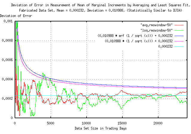
Figure X is a plot of the deviation of the error in the measurement
of the mean of the marginal increments,
avg, by averaging and least squares fit
on the fabricated data set with a mean of exactly 0.000232 and a
deviation of 0.010988. It was produced using the tsrmswindow
program, (using the -w 50 option,) on the data presented in Figure IX
and represents the deviation of the error vs. the data set size. The
interpretation of Figure X is that, for example, at 5000 trading days,
the deviation of the error in the measurement of the mean would be
about +/- (0.0004 - 0.000232) = 0.000168
for one standard deviation of the time, or (double sided,) about
68.27% of the time. The error convergence should follow an
rms * erf (1 / sqrt (t)) function as in
Bernoulli
P Trials, where t is the data set
size, and rms is the deviation of the
marginal increments. For t >> 1,
erf (1 / sqrt (t)) is approximately
1 / sqrt (t).
For example, the deviation of the error for the DJIA, with a data
set size of 24,048 elements would be approximately
0.010988 / sqrt (24048) =
0.000070856414
, and 0.000070856414 /
0.000232 = 0.305415578 which agrees favorably with the
statistical
estimates presented above.
So, as an approximation, letting avg
and rms be the average and deviation,
respectively, of the marginal increments of a time series that has
n many elements, the deviation of the
error in the measurement of avg will be
(rms / avg) / sqrt (n).
(Its an interesting equation, see Section
I where it is shown that avg and
rms are all that are required to define
the investment quality of an equity-which can be compensated for data
set size using this technique.)
The conclusions drawn in Addendum II and Addendum III were drawn on local characteristics-by analyzing data in the recent past.
But what if the recent decline was the beginning of a significant decline in the US equity market indices? What if the decline in investor confidence deteriorated indefinitely?
Equation
(1.20) from Section
I, the exponential marginal gain per unit time,
g:
                 P          (1 - P)
    g = (1 + rms)  (1 - rms)        ....................(1.20)
and, Equation (3.1) from Section III, the deviation of an indices' value from its median:
rms * sqrt (t) .....................................(3.1)
can yield some insight into the characteristics of significant
declines in the values of indices. For convenience,
g is converted to an exponential
function, e^t ln (g). Then the formula
for the negative deviation of an index from its median value, from Section
III, Figure
I, would be:
e^((t * ln (g)) - (rms * sqrt (t))) ................(A.1)
In a significant decline, for one standard deviation of the time, (about 84% of the time,) an index will be above the values in Equation (A.1), and below 16%. As an alternative interpretation, 84% of the declines will not be as severe as the values in Equation (A.1), and 16%, worse.
Note that the negative deviation is e^((t * ln (g)) -
(rms * sqrt (t))), and two negative deviations are
e^((t * ln (g)) - (2 * rms * sqrt (t))),
and so on.
Equation (A.1) has a certain esthetic appeal-it consists of three functions: a linear term; a square root term; both of which are exponentiated. In some sense, the linear term represents the fundamentals of the equities in an index, (and is probably a macro/microeconomic manifestation,) and the square root function represents the fluctuations in the index value do to speculation-it is the speculative risk as a function of time, and is probabilistic in nature. The exponentiation function is an artifact of the geometric progression of the index value-it represents the way the index is constructed, from one time period, to the next, and is stable in the sense that it is a multiplication process, which is the same for each and every time period.
|
As a side bar, all the paragraph says is that for each time
period, get a Gaussian/Normal unit variance random number;
multiply it by Equation (A.1) is the deviation from the median value of an
index constructed by such a process where the term |
The historical time series of the DJIA, NASDAQ, and S&P500
indices through December 5, 2002 was obtained from Yahoo!'s database of equity Historical Prices, (ticker
symbols ^DJI, ^IXIC, and, ^SPC,
respectively,) in csv format. The csv format was
converted to a Unix database format using the csv2tsinvest
program. (The DJIA time series started at January 2, 1900, the NASDAQ
at October 11, 1984, and January 3, 1928 for the S&P500.)
The values for avg and
rms for each index was derived using the
tsfraction
program, and piping the output to the tsavg
and tsrms
programs using the -p option,
respectively.
P, in the time series of each index:
        avg
        --- + 1
        rms
    P = ------- ........................................(1.24)
           2
from Section I, and Equation (A.1) plotted for each index, with the two significant declines in the index values in the last one hundred years-September 3, 1929 through November 23, 1954, and, January 14, 2000 through December 5, 2002, (which may not be over yet.) On September 3, 1929, the DJIA was at its maximum value before the Great Depression-it did not increase above that value until November 23, 1954. The DJIA was at its historical maximum value on January 14, 2000.
Both declines are plotted for the DJIA, S&P500, and, NASDAQ by rescaling the index values to unity at the beginning of each decline, along with the deviation of the indices from Equation (A.1).
For the DJIA, (using the complete 28140 trading day data set
from January 2, 1900 to December 5, 2002,) the mean of the marginal
increments, avg, of the time series,
was 0.000233, and the deviation,
rms, of the marginal increments,
0.011028, giving the probability of an
up movement, from Equation
(1.24), in the DJIA, P, of
0.51056401886, and, from Equation
(1.20), a daily gain in value, g,
of 1.00017221218, or, from Equation
(A.1), the negative deviation of the DJIA:
e^((t * ln (1.00017221218)) - (0.011028 * sqrt (t)))
For the NASDAQ, (using the complete 4582 trading day data set
from October 11, 1984 to December 5, 2002,) the mean of the marginal
increments, avg, of the time series,
was 0.000487, and the deviation,
rms, of the marginal increments,
0.014448, giving the probability of an
up movement, from Equation
(1.24), in the NASDAQ, P, of
0.516853544, and, from Equation
(1.20), a daily gain in value, g,
of 1.00038272386, or, from Equation
(A.1), the negative deviation of the NASDAQ:
e^((t * ln (1.00038272386)) - (0.014448 * sqrt (t)))
For the S&P500, (using the complete 19896 trading day
data set from January 3, 1928 to December 5, 2002,) the mean of the
marginal increments, avg, of the time
series, was 0.000262, and the
deviation, rms, of the marginal
increments, 0.011367, giving the
probability of an up movement, from Equation
(1.24), in the S&P500, P, of
0.51152458872, and, from Equation
(1.20), a daily gain in value, g,
of 1.00019742225, or, from Equation
(A.1), the negative deviation of the S&P500:
e^((t * ln (1.00019742225)) - (0.011367 * sqrt (t)))
|
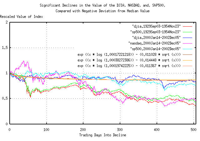
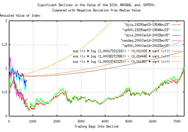
Figure XI is a plot of the declines in the US equity indices, (September 3, 1929, through, November 23, 1954, for the DJIA, S&P500, and, January 14, 2000, through, December 5, 2002, for the DJIA, S&P500, and, NASDAQ,) and the deviation from the median, from Equation (A.1), for all three indices. The first 506 trading days of the decline are shown-about two calendar years.
Of interest is the DJIA and S&P500 from January 14, 2000, through, December 5, 2002 tracking their deviation values; the current decline of the DJIA and S&P500, during the first two years, seems to be a somewhat typical significant decline, (the deviation being regarded as the definition of typical.)
However, the DJIA and S&P500 faired much worse, comparatively, during the first 50 days of decline after September 3, 1929, as did the NASDAQ in the first 506 days of the decline that started on January 14, 2000.
|
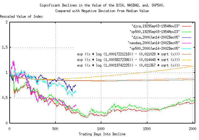
Figure XII is a plot of the declines in the US equity indices, (September 3, 1929, through, November 23, 1954, for the DJIA, S&P500, and, January 14, 2000, through, December 5, 2002, for the DJIA, S&P500, and, NASDAQ,) and the deviation from the median, from Equation (A.1), for all three indices. The first 2024 trading days of the decline are shown-about eight calendar years.
Of interest is the DJIA and S&P500 from January 14, 2000, through, December 5, 2002 still, approximately, tracking their deviation values. Note that the DJIA and S&P500, September 3, 1929, through, November 23, 1954, bottomed on trading day 843, (on July 8, 1932,) at close to five times its deviation value, (i.e., a five sigma hit,) and that the DJIA and S&P500 bottomed about where their deviation from their median values bottomed-around a thousand trading days, or four calendar years-and that the curves have the same shape, (although the relative magnitudes are different.)
Also, note that the bottoms of the deviation from the median values occur at different times-the NASDAQ being first; the DJIA being last. Its a consequence of the values of the variables in the deviation equations-there is no merit in assuming that index declines bottom in a prescribed way; like in so many years into the decline, etc.
|
Figure XIII is a plot of the declines in the US equity indices, (September 3, 1929, through, November 23, 1954, for the DJIA, S&P500, and, January 14, 2000, through, December 5, 2002, for the DJIA, S&P500, and, NASDAQ,) and the deviation from the median, from Equation (A.1), for all three indices. The full 7297 trading days of the decline are shown-almost twenty nine calendar years.
Of interest is the shape of the DJIA and S&P500 September 3, 1929, through, November 23, 1954 curves-and how they are similar to their deviation from median values for the 29 year period.
Note that this analysis is, in some sense, a worst case scenario-where the decline in investor confidence deteriorated indefinitely; for almost 30 years. The negative deviation is actually a probability envelope. As shown in Addendum II and Addendum III, the value of an index wanders around, between its positive and negative deviation-around the median-for one standard deviation of the time. In the worst case scenario, positive recovery back to the median value is delayed, indefinitely.
As a simple high entropy model of political polls where candidates jockey for position in favorability ratings by stumping-sometimes a message is received well, and sometimes not-simple fractal dynamics can be used to analyze the probabilities of an election's outcome.
On August 12, 2003, the polls, (ref: NBC News, August 11, 2003,) indicated that there was a 59% chance of California Governor Gray Davis being recalled. If the recall was successful, the two top candidates to replace Davis are Cruz Bustamante-the current California Lieutenant Governor-with a 18% favorability rating, and the actor, Arnold Schwarzenneger, with a 31% favorability rating. Analyzing many political polls, the deviation of favorability ratings is about 2% per day-meaning that the daily movement in a favorability rating will be less than +/- 2% one standard deviation of the time, which is about 68% of the time.
A simple fractal model of favorability polls would be to start at
some initial point, (18% for Bustamante, 35% for Schwarzenneger,) and
then add a number from a random process, (a Gaussian/Normal
distribution is assumed-with a deviation of 2%,) for the next day's
poll number, then add another number from the random process for the
day after that, and so on-i.e., a simple Brownian motion fractal. This
means that the deviation of the pole ratings
n many days from now would be
2 * sqrt (n) percent, as shown in Figure
XIV.
|
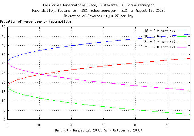
Figure XIV is a plot of the deviation of Bustamante's and
Schwarzenneger's favorability polls, projected to the election day,
October 7, 2003, based on poll data taken on August 11, 2003. The
interpretation of the graph, using Bustamante as an example, is that
the deviation of Bustamante's favorability on October 7 would be
2 * sqrt (57) = 13%, (October 7, 2003,
is 57 days into the future from August 12, 2003,) meaning that on
October 7, there is a one standard deviation chance, about 84%, that
Bustamante's favorability will be less than 18 + (2 *
sqrt (57)) = 33%, and an 84% chance that it will be
greater than 18 - (2 * sqrt (57)) =
3%. Likewise for Schwarzenneger's poll ratings.
Also, up to October 7, 2003, the poll ratings for each candidate
will be inside of the +/- 2 * sqrt (n)
curves 68% of the time-and above it 16% of the time, and below it 16%
of the time. Additionally, the poll numbers will be characterized by
fluctuations that have probabilistic durations of erf (1
/ sqrt (n)) which is approximately 1 /
sqrt (n)) for n >>
1. For example, what are the chances that
Schwarzenneger's favorability rating of at least 31% continuing
consecutively over at the next 57 days to the election? It would be
about 1 / sqrt (57) = 13%.
|
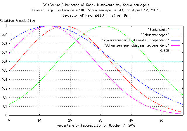
Figure XV is a plot of the favorability rating probabilities for
Bustamante and Schwarzenneger on October 7, 2003, based on poll data
taken on August 11, 2003. The deviation of both is 2 *
sqrt (57) = 15%. However, to get the probabilities of
an election win for both candidates, subtract both-and there are two
ways of doing it; assume the distributions are statistically
independent, (i.e, the resulting distribution has a deviation of
sqrt (2) * 2 * sqrt (57) = 21%,) or,
assume the distributions are dependent, (i.e., the resulting
distribution has the same deviation, 2 * sqrt (57) =
15%, assuming the poll ratings are a zero-sum
game-what one candidate gains, the other loses.) Both of the resulting
distributions center on 31 - 18 = 13%,
and one has a deviation of 21%, the other, 15%. For a win, the
probabilities must be positive, or for a dependent/zero-sum
interpretation, Schwarzenneger has about a 73%, (13 / 21
= 0.62 single sided deviation, which is about 27%,)
chance of beating Bustamante on October 7. For the statistically
independent interpretation, it is about 81%, (13 / 15 =
0.87 single sided deviation, which is about 19%.) The
real probability probably lies somewhere between the two, at about
75%.
For Davis to beat the recall, he must make up at least 9% in
favorability, or a 9 / 15 = 0.6
deviation, which is a 27% probability.
Bear in mind that these probabilities are projected from poll data taken on August 11, 2003, and a lot can change. But as of August 11, the probabilities are:
Note, also, that the chances of California having a Democratic
governor on October 7, 2003, is 25% + 27% =
52%, too.
Another useful fractal tool in analyzing poll data is the Gambler's
Ultimate Ruin. What are the chances, assuming that stumping is a
zero-sum game-probably meaning mud slinging-of Schwarzenneger beating
Bustamante in a landslide? (31 / 2) / ((31 / 2) + (18 /
2)) = 63%, and it would take (18 / 2)
((31 / 2) - (18 / 2)) = 58 days, on average, (the
division by 2 is for formality, because the "currency" of the game is
2% in poll ratings per day.) How about Bustamante beating
Schwarzenneger in a landslide? 37%, and
it would take 101 days, on
average. Note, from Figure XV, that it is to Bustamante's advantage to
drive the contest to a zero-sum game, where he has an 27% chance of
winning, versus a 19% chance if he doesn't. Likewise, it is to
Schwarzenneger's advantage to avoid playing the contest as a zero-sum
game-he would have 8% less in poll ratings to make up.
As an historical note, California Recalls are not uncommon-there have been 118 recall attempts in the 93 year history of the the Amenement; four of them for govenors, Edmund G. "Pat" Brown Ronald Reagan Edmund G. "Jerry" Brown Pete Wilson, all of which failed.
The assumption that favorability poll data is characterized as a Markov-Wiener process is similar to the assumptions made by Black-Scholes-Merton about equity prices; the marginal increments are statistically independent, and have a Gaussian/Normal distribution-ignoring leptokurtosis and log-normal evolution of a candidate's poll ratings.
Most political economists argue that leptokurtosis in social systems is the rule, and not the exception. An interpretation is that things go steadily along-with a reasonable amount of uncertainty-and then, spontaneously there is a jump of many standard deviations. The jumps tend to cluster, and are characteristic of social change, (for example, during insurgence/rebellion/revolt, jumps in the range of orders-of-magnitude many standard deviations are common; yet-using the mathematics that are used by pollsters-such occurrences have a probability that is indistinguishable from zero.)
There is cause for concern in the accuracy of the poll numbers, (or
there are some self-serving polls being published.) Bustamante's
favorability was 18% on August 11, 2003, and on August 24, 2003, it
was 35%, (ref: the Los
Angeles Times.) What's the chances of a move to 35% in about 15
days? The standard deviation of the chance is 0.02 *
sqrt (15) = 7.7%, and 35 - 18 /
7.7 is 2.2 standard
deviations, which is a chance of 1.4%. Not a very likely occurrence,
(not impossible, but not very likely, either.) Such things are a
hallmark signature of leptokurtosis in the daily movements of the
favorability numbers-meaning that there are "fat tails" in the
distribution of the movements. This implies the volatility is a factor
of 2.2 what would be measured as the deviation of the daily movements,
(the metric of volatility is the deviation of the movements, where
volatility is interpreted as risk, or uncertainty; similar to the
classic definition of Black-Scholes-Merton's
"implied
volatility.")
There is probably something else that is going on besides the
recall of the California Governor. At least that's what the poll
numbers tend to indicate. (With a 100 - 1.4 =
98.6% certainty.)
|
As a side bar, whatever else is going on besides the recall of the California Governor seems to concern the California Budget. California is currently running at a deficit of $38 billion; down from a $10 billion surplus when Gray Davis became Governor four years ago. Deficits in California are not that unusual-the last California Administration to run a sequence of surpluses was run by Governor Earl Warren, 1943-1953. But state budgets can be optimized-there exists a budget solution that maximizes commitments to future spending, while at the same time, minimizing the risk of the commitments of the spending. Using the US GDP as an example, from the analysis of the US
GDP, above, the quarterly average, A spending growth less than Obviously, different states have different optimizations, but Davis' spending between 1999 and 2004 increased by 36%, while tax revenues increased by 28%-and that was because of an economic bubble, (which should have been handled differently, see the US GDP of Section III for particulars.) Whatever else is going on besides the recall of the
California Governor seems to have a lot of the
characteristics of a revolt-with a
|
Note: this appendix originated in the NtropiX and NdustriX mailing lists in August, 2003. See:
for the originals.
Wars tend to be an high entropy affair, (as illustrated by Clauswitz's "fog of war" statement-meaning that the future outcome of a military interdiction is uncertain,) so, one would expect about half the wars, on an an annual time scale, to last less than 4.3 years, and about half more-where the wars are made up of a series of battles, large and small, each with an outcome that is uncertain, (i.e., a fractal process.) History seems to support the conjecture, (for example, the chances of a hundred year war/Boer war is about 1 in sqrt (100) = 1 in 10, and most last somewhat over 4 years.) Its a direct consequence of Equation (3.1) in Section Section III.
So, for a typical war, the situation would deteriorate for
about half the 4.3 years, bottoming at about 2 years, and a military
decision would be concluded in somewhat over 4 years, (whatever the
term typical war means.) The probability of it continuing at
least t many years would be
erf (1 / sqrt (t)) which is about
1 / sqrt (t) for t
>> 1.
Since war is a high entropy system, the Gambler's
Ruin can be used to calculate the chances of the combatants
winning. Suppose one combatant has x
resources, and the other y. Then the
chances of the latter winning is y / (x +
y), (which says to engage a combatant with much less
resources-another of mathematics most profound insights-but at least a
number can be put on it.) The duration of the war would be
y * (x - y) battles, (since that is the
currency of war,) for x > y.
Note that even if one combatant has significantly more resources than any other and iterates enough wars, eventually, the combatant will go bust, and lose everything-war is at best, (if one can have a war with no death or destruction,) a zero-sum game; what one side wins, the other loses.
|
As a side bar, for a zero-sum game, it is a necessary, but insufficient, requirement that "what one side wins, the other loses." If war was as simple as that, no one would make war, (the strategic outcomes of fair iterated zero-sum games is that neither player wins in the long run.) For a formal zero-sum game, the player's utilities must be considered-in the case of war, the utility is to resolve a question of authority. |
43 days before the election:
The recent polls say 46% of the voters, (in the popular vote,) would vote for Bush, 43% for Kerry. There are 43 days left to the election, and the polls move at about 1% per day, and are a zero-sum game, (in the simple/lay sense-what Bush gets in a poll on one day, Kerry loses, and vice verse, ignoring the formalities of utility.)
What that means is that
sqrt (43) = 6.5574385243%is the standard deviation of the popular vote poll data on election day-43 days from now-or there is a 14% chance that Bush's poll data will be above46 + 6.5574385243 = 52.6%, and a 14% chance of being below46 - 6.5574385243 = 39.4%. The numbers for Kerry on election day is a 14% chance of being above43 + 6.5574385243 = 49.6%and a 14% chance of being below43 - 6.5574385243 = 36.4%.Since it is a zero-sum game, the winner of the popular vote will have to have more than
43 + ((46 - 43) / 2 ) = 44.5%, or a1.5 / 6.5574385243 = 0.228747855standard deviations.Referring to the CRC tables for the standard deviation, 0.228747855 corresponds to about a 59% chance for Bush, and a 41% chance for Kerry, to win-call it a 60/40 chance, 43 days from now.
25 days before the election:
The +/- 3 points margin of error is a statistical estimate of the accuracy of the poll; its the estimated error created by sampling the population-which is used to generate the poll numbers. It means that the "real" value of the aggregate population lies between a 52% for one candidate and 46% for the other, for one standard deviation of the time, or about 68% of the time, (and it would be more than a 52% win and less than a 46% loss for 16% of the time for one candidate, and 16% of the time for the other, too.)
So, what does it mean for the election 25 days away?
The statistical estimate is an uncertainty, and the uncertainty will increase by about
sqrt (25) = 5%by election day, (relative to today,) meaning that the standard deviation on election day will be +/- 8%, or there is a 16% chance that Bush will win by more than 57% to Kerry's 41%, and likewise for Kerry. The chances of them being within +/- 1% on election day is one eighth of a standard deviation, or about 10%, (one eighth of a standard deviation is about 5%, but it can be for either candidate, or +/- 1%.)The new Reuters/Zogby poll was just released:
- http://www.zogby.com/news/ReadNews.dbm?ID=877
and Bush has a 46% to 44% advantage over Kerry in the popular vote as of today, with a +/- 3% statistical estimate in the sampling accuracy.
Using that data, and considering the election is 25 days away, (or the distribution on election day would be about the
sqrt (25) = 5%,) Bush would have a2 / 5 = 0.4standard deviation of winning, or about 66%, (note that the chances of Bush winning increased since September 21, when he had a 3% advantage over Kerry, and only a 2% today.)Including the +/- 3% uncertainty of the sampling error, (and using a Cauchy distribution for a worst case-not so formal-estimate,) the "standard deviation" would be +/- 8%, Bush would still have a
2 / 8 = 1 / 4standard deviation, (we really should use the median and interquartiles,) or about a 60% chance of winning. (Considering the distributions to be a Cauchy distribution-we add them linearly since Cauchy distributions are highly-actually the maximum-leptokurtotic, with a fractal dimension of 1.)Or, if we consider the distributions to be Gaussian/Normal, (i.e., we add the root-mean-square of the distributions root mean square; it has a fractal dimension of 2,) then the distribution on election day would be
sqrt (3^2 + 5^2) = 5.8, or about 6%. Then Bush's chance of winning would be2 / 6 = 1 / 3standard distribution, or about 63%.So, Bush has between a 60 and 63 percent chance of winning, (these are the two limits-between no leptokurtosis and maximum leptokurtosis,) probably laying closer to 63%, including the uncertainty of the sampling error, and making no assumptions about leptokurtosis.
1 day before the election:
The movements in polls have high entropy short term dynamics, and if one candidate is ahead the chances of the candidate remaining ahead for at least one more day is
erf (1 / sqrt (t)), where t is the number of days the candidate has already been ahead.Or, the chances of Bush's short term lead continuing through tomorrow, November 2, is
erf (1 / sqrt (4)) = 0.521143, which is very close.
Note: this appendix originated in the NtropiX and NdustriX mailing lists in September, October, and November, 2004. See:
for the originals.
The Social Security Trustees Middle Projection for the date of Social Security insolvency is 2042-37 years from now; it is based on the assumption of a US GDP median growth rate of 1.8% per year. How realistic is that assumption?
Using the analysis of the US
GDP, above, the quarterly average, avg =
0.008525, and deviation, rms =
0.013313, of the marginal increments of the US GDP
would give the chances of an up movement in the US GDP,
P = ((avg / rms) + 1) / 2 = 82% in any
quarter, for a quarterly GDP expansion of
1.008472, (from Equation (1.18)
in Section
I.)
Converting to annual numbers, for convenience, the annual deviation
of the US GDP would be about rms = sqrt (4) * 0.013313 =
0.026626, and the median annual expansion would be
about 1.008472^4 =
1.03432108616. Meaning that 27 years from now, the
median value of the US GDP would be 1.03432108616^27 =
2.48711129433 what it is today, about ten trillion
dollars.
Converting the US GDP data to its Brownian motion/random walk
fractal equivalent, as described in Section
II, the annual linear gain of the US GDP would be about
ln (1.03432108616) = 0.0337452561, which
would have a value of 27 * 0.0337452561 =
0.911121914 in 27 years.
The deviation of the US GDP around its average value of
0.911121914 would be about
sqrt (27) * 0.026626 = 0.138352754 in 27
years.
For the Social Security Trustees Middle Projection, the equivalent
value of the US GDP in 27 years would be ln (1.018) * 27
= 0.48167789.
So, how realistic is the Social Security Trustees Middle Projection assumption on what the US GDP will be 27 years from now?
There is a (0.911121914 - 0.48167789) / 0.138352754 =
3.10397886261 standard deviation chance of it-or a
chance of 0.000954684857590260, (about a
tenth of a percent,) which is about one chance in a thousand, that the
US GDP, 27 years from now, will be as bad, or worse, than their
assumption.
A very conservative assumption, indeed.
Multiplayer election polls are, at best, numerology-and projecting election winners can be difficult. As a non-Linear high entropy system model, each of the players vie for the most votes by gambling on the votes they already have, (i.e., their rank in the polls.) To gain in the ranking, a risk must be taken to say, or promise, something, (truthful or not,) that will alienate some of the votes a candidate already has, in hope of getting more votes from a competitor than is lost-which might be a successful ploy, or might not. As the players jockey for position in the polls, over time, each player's pole values will be fractal. Some straight forward observations:
A player's pole value can never be negative.
A pole value can, effectively, be greater than 100% at election time, since the voter turn out, (which is very difficult to forecast-it depends on things like the local weather,) can be more than expected, (i.e., population increase, volatile issues that polarize the electorate-enhancing voter turn out, etc.)
This means that the pole values for the players will evolve into a log-normal distribution, (see: Section II for particulars,) and the players are wagering a fraction of the voters they have in hopes of gaining more, which sometimes works out, and sometimes doesn't, (i.e., the fractals are geometric progressions.)
Note that this model is identical to the model for equity prices, except that the currency is percentage points of favorability.
|
As a side bar, the NdustriX, Utilities
can be used for a precise estimation of election outcomes, as can
the |
As an alternative, the log-normal distribution algorithms used in
the tsinvest
program were used in the poll
program, (the sources are available at poll.tar.gz
as a tape archive,) which will be used in the analysis.
The, data, as an example, ranking the Democratic candidates is from http://www.usaelectionpolls.com/2008/zogby-national-polls.html, and was taken on 10/26/2007, (Zogby America Poll):
The Margin of Error was 4.1%.
Note that the rankings have evolved, (approximately,) into a log-normal distribution, (the ratio of the value of one rank, divided by the value of the next rank, for all the ranks is approximately constant-about a factor of 2-the hallmark signature of a log-normal distribution.)
Rather than use the empirical data, typical values will be used, (leaving the real data as an exercise in intuition for the reader):
And we will assume the election is to be held 90 days from now, and the deviation of the day-to-day ranking values is about 2%, which is a typical number for election polls:
  poll -N -t 90 -r 2 50 25 12.5 6.25 6.25
  Player 1's chances of winning = 0.891711
  Player 2's chances of winning = 0.089691
  Player 3's chances of winning = 0.011935
  Player 4's chances of winning = 0.003331
  Player 5's chances of winning = 0.003331
Which assumes a Gaussian/normal distribution evolution of the rankings, (note that Player 1, at a 90% probability of winning, is almost a certain winner, against second place which has only a one chance in ten of winning.)
Including the -l option to the poll program to evaluate the probabilities of each player winning with a log-normal distribution evolution fractal:
  poll -l -N -t 90 -r 2 50 25 12.5 6.25 6.25
  Player 1's chances of winning = 0.522636
  Player 2's chances of winning = 0.266320
  Player 3's chances of winning = 0.118930
  Player 4's chances of winning = 0.046057
  Player 5's chances of winning = 0.046057
And, Player 1 has a far less certain chance of winning of about a one in two chance, (and Player 2 has about a one chance in four of winning.)
Such is the nature of log-normal distributions.
A note about the model used in the analysis.
If there are only two players, then the two distributions of the players poll rankings are not independent, (the model used in the analysis assumed not only independent but iid.) In point of fact, if there are only two players, the poll values are a zero-sum game, (i.e., what one player gains, the other loses-a negative correlation.)
The algorithm used in the analysis assumes that there are sufficiently many candidates, and there is an equal probability of any player gaining in poll value at the expense of any of the other players.
Real elections lie between these two limits.
The historical time series of quarterly housing prices for
Sunnyvale California, from 1975 Q4 through 2007 Q4, inclusive, (about
a third of a century,) was obtained from the Office of Federal Housing Enterprise
Oversight, (file,) and
edited with a text editor to make a time series,
san_jose-sunnyvale.txt.
The time series data set size is only 129 data points-which is only marginally adequate for analysis, and appears to be smoothed, (probably a 4 quarter running average,) which, unfortunately, is common for government supplied data.
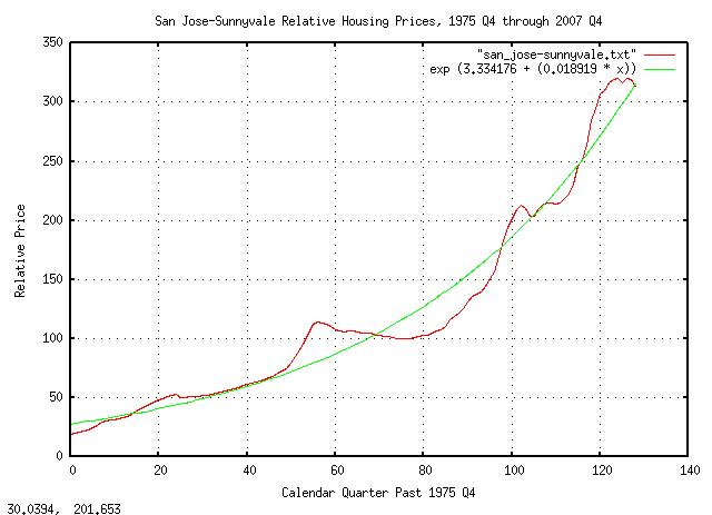
Calculating the least squares, (LSQ,) exponential best fit of the data:
    tslsq -e -p san_jose-sunnyvale.txt
    e^(3.334176 + 0.018919t) = 1.019100^(176.229776 + t) = 2^(4.810199 + 0.027295t)
|
Figure XVI is a plot of quarterly housing prices for Sunnyvale California, from 1975 Q4 through 2007 Q4, inclusive, and its exponential LSQ best fit. Over the third of a century, housing prices increased an average of 1.9% per calendar quarter, which corresponds to 7.9% per year.
|
As a side bar, the the DJIA averaged an annual growth rate of about 9.4% over the same time interval, (and note that equity values can be defended in times of uncertainty with a stop loss, order i.e., taking a "short" on an equal number of shares of stocks-which can not be done with residential housing assets.) The average annual inflation rate, (using US Government deflation time series,) over the time interval was about 4.7% per year. Note that the stagflation of the early 1980's, (about the twentieth quarter in the graph,) is clearly visible in housing prices, which increased only moderately in an era of double digit inflation-and mortgage interest rates. Note, also, that the recession of the early 1990's is visible, (about the sixtieth quarter in the graph,) and housing prices remained below their median long term value for almost 5 years, increasing into the current bubble, (with a slight downturn in the early 2000's equity market uncertainty, at about quarter 110.) Bubbles in asset prices are common-and their characteristics will be analyzed, below. Large historical asset devaluations, although not common, are not unheard of, either. During the US Great Depression, (1929-1933,) assets lost 60% of their value, (and the DJIA lost 90% of its value-not recovering until 1956-and the US GDP dropped 40%.) Fortunately, such occurrences are rare; about once-a-century events, (but the chances of such an occurrence happening during the time interval of a thirty year mortgage can not be ignored-about one in three.) More recently, the crash in asset prices in Japan during the early 1990's created a devaluation of about 40% in property prices. (See Asset price declines and real estate market illiquidity: evidence from Japanese land values, or the referenced PDF paper from the Federal Reserve Bank of San Francisco.) |
Generating the quarterly marginal increments of housing prices:
    tsfraction san_jose-sunnyvale.txt | tsnormal -t > san_jose-sunnyvale.frequency
    tsfraction san_jose-sunnyvale.txt | tsnormal -t -f -s 17 > san_jose-sunnyvale.distribution
|
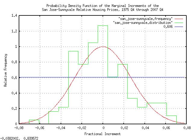
Figure XVII is a plot of the quarterly marginal increments of housing prices in Sunnyvale, California, from 1975 Q4 through 2007 Q4, inclusive. Note, (even for such a small data set size,) the increment's probability distribution function, (PDF,) is approximately Gaussian/Normal. This is to be expected from the Central Limit Theorem, (and means we are probably dealing with a non-linear high entropy system; a fractal.) All it means is that the probability of a large change in asset value, from one quarter to the next, is less than a small change.
Generating the probability of the run lengths of expansions and contractions of housing prices:
tsmath -l san_jose-sunnyvale.txt | tslsq -o | tsrunlength | cut -f1,5 > san_jose-sunnyvale-runlength
|
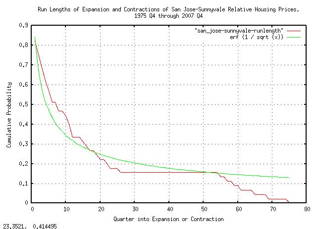
Figure XVIII is a plot of the distribution of the durations of the
expansions and contractions in housing prices in Sunnyvale,
California, from 1975 Q4 through 2007 Q4, (only the distribution of
the positive run lengths are shown.) Also, the fractal theoretical
value, erf (1 / sqrt (t)), is
plotted for comparison.
|
As a side bar, note that the half of the expansions and contractions lasted less than 4.3 quarters, and half more. Also, even with the limited data set size, there is reasonable agreement between the empirical data and theoretical fractal values. The graph in Figure XIII expresses, probabilistically, how long
a contraction, (or expansion,) will be. For Fractals are self similar, meaning that the graph in Figure XIII does not change if the time scale is changed. The same probabilities hold true. For example, what are the chances that a contraction will last 10 years? About 31%. A hundred years? About one in ten. (That's why they are called fractals.) Probably the best way to conceptualize asset values as fractals is to consider them made up of bubbles which are made up of smaller bubbles, which in turn are made up of even smaller bubbles, ..., without end, at all scales. For example, a contraction that lasts 100 years would be made of smaller expansions and contractions, which are made up of ... But the smaller expansions and contractions would not be sufficient to end the 100 year contraction, before its time. That's what the graph in Figure XIII illustrates-it is simply a probability distribution function of the duration of the expansions and contractions in housing prices. The important concept is that if any time scale is chosen, (say
years,) then half the contractions and expansions will last less
than 4.3 years, and half more, ( |
Addressing the magnitude of the expansions and contractions, which are dependent, (approximately,) on the root-mean-square of the increments of the housing prices:
    tsmath -l san_jose-sunnyvale.txt | tslsq -o | tsderivative | tsrms -p
    0.025923
And the root that should be used:
    tsmath -l san_jose-sunnyvale.txt | tslsq -o | tsrootmean -p | cut -f2
    0.794815
For generating the theoretical fractal values,
0.025923 * (t^0.794815), and analyzing
the empirical values:
tsmath -l san_jose-sunnyvale.txt | tslsq -o | tsrunmagnitude -r 0.794815 > san_jose-sunnyvale-runmagnitude
|
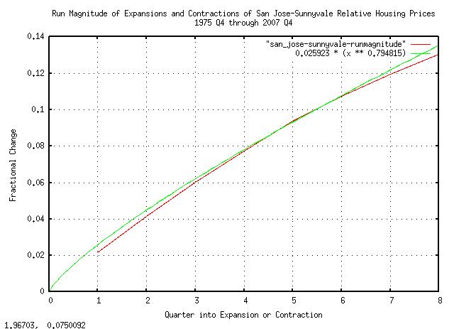
Figure XIX is a plot of the magnitude of the expansions and contractions in housing prices in Sunnyvale, California, from 1975 Q4 through 2007 Q4, and its theoretical fractal values.
|
As a side bar, a root of With that said, what the graph in Figure XIX means is that in
|
Note that the housing prices are currently at parity with the long
term value, (the green line in Figure XVI,) as of Q4, 2007, and seems
to be 16%, or so, below the value at the peak of the
bubble. How much further will they go down using a calendar
year for the time scale? There is a 50/50 chance that prices will
return to parity, (the green line in Figure XVI,) within 4.3 years,
(and a 50/50 chance they won't.) How much will the prices decrease?
If it is a typical contraction, then prices will decrease for
about two years, then increase for two years, back to parity. In two
years, there is a 16% chance that prices will deteriorate by more than
a factor of 0.92^2 = 0.85 ~ 14% of their
current value for a total of a 31% decline from the peak of the
bubble, (and an 84% chance that the price deterioration will
be less.)
Taken together, the chance that the current contraction that will
last less than 4.3 years, and, the chance that the price deterioration
will be less than 31% from the peak of the bubble, is a
combined chance of 0.84 * 0.5 = 0.42 =
42%, (and a 58% chance that it will be worse.)
|
As a side bar, to calculate the optimal "margin" on an investment, consider the "standard" equations: which is optimally maximum when: Where: from the first equation. Now, consider investing in something-like a residential
property-which has a total price, Optimality, occurs when: where This solution is optimal in the sense that the growth in the equity value, (the down payment,) is maximized, while at the same time, minimizing the chances of a future negative equity value, (i.e., the value of the house going "underwater".) For San Jose-Sunnyvale, CA, the optimal down payment would be about 22% of the value of the property. (Significantly less than 22% down would increase the chances of the property being "underwater" in the first few years of the mortgage, and more than 22% down would reduce the annual ROI on the down payment.) |
The historical price per barrel of light sweet crude oil futures
was downloaded from http://www.eia.doe.gov/emeu/international/crude2.html,
and Contract 1, (i.e., future price for delivery in the next calendar
month,) was edited with a text editor to make a time series,
crude2.
    tslsq -e -p crude2.txt
    e^(2.620487 + 0.000625t) = 1.000626^(4189.645647 + t) = 2^(3.780564 + 0.000902t)
|
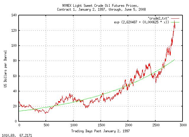
Figure XX is a plot of the the NYMEX Light Sweet Crude Oil Futures Prices, Contract 1, January 2, 1997, through, June 5, 2008. Note that the price is in a bubble, (over valued by about 60%,) which is not uncommon in non-linear high entropy economic systems; in a typical year, the ratio of the maximum price to the minimum will be about a factor of two.
Note that the price of light sweet crude has increased at about a 15% per year rate over the last decade, (compared with an increase in equity values-using the DJIA as a reference-over the Twentieth Century of 5-7% per year, or an increase in the US GDP of about 4% a year.) The increase in the price of light sweet crude and the DJIA are not adjusted for inflation; the US GDP, however, is in real dollars. US Inflation over the last decade averaged about 3-4% per year. The value of the dollar has fallen about 30% over the decade-although foreign oil is purchased in US dollars, those dollars must be, eventually, converted to a foreign currency, and it will take about 30% more dollars to do so today than a decade ago. All-in-all, the price of light sweet crude has increased about 5-7% per year over the last decade, (in real dollars,) which is commensurate with the inflation in crude oil, world wide.
Note, also, that the price of crude oil is determined by the futures traders, and not the oil companies, (the oil companies "buy" oil from the traders-for a given price, at a given time in the future.)
    tsfraction crude2.txt | tsavg -p
    0.000830
    tsfraction crude2.txt | tsrms -p
    0.023151
The price volatility of crude has a standard deviation of 2.3151
percent per day, (which is about twice the the DJIA's was over the
Twentieth Century,) meaning the risk is about twice as high-as a short
term investment. But note the efficiency of the increase in price-if
the average increase was 0.023151^2 =
0.000536, the growth in price would be
maximal. An efficiency of 0.000536 / 0.000830 =
65% is a typical characteristic of an expanding
competitive, capital intensive, market.
    tsfraction crude2.txt | tsnormal -t > crude2.frequency
    tsfraction crude2.txt | tsnormal -t -f > crude2.distribution
|
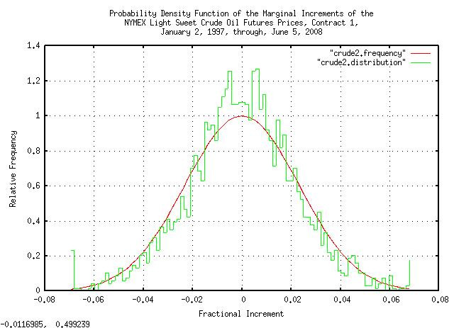
Figure XXI is a plot of the probability density function of the marginal increments of the NYMEX light sweet crude oil futures prices, contact 1, January 2, 1997, through, June 5, 2008. Notice how well the the empirical data matches the theoretical data.
tsmath -l crude2.txt | tslsq -o | tsrunlength | cut -f1,5 > crude2-runlength
|
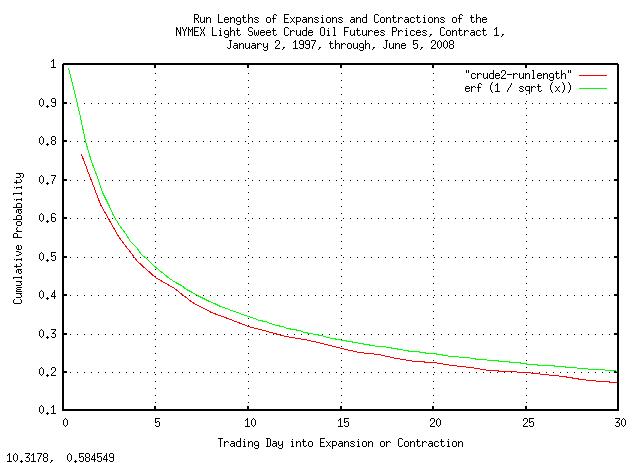
Figure XXII is a plot of the run lengths of expansions and contractions of the NYMEX light sweet crude oil futures prices, contract 1, January 2, 1997, through, June 5, 2008. Again, notice how well the the empirical data matches the theoretical data.
tsmath -l crude2.txt | tslsq -o | tsderivative | tsrms -p
0.023181
tsmath -l crude2.txt | tslsq -o | tsrootmean -p | cut -f2
0.498672
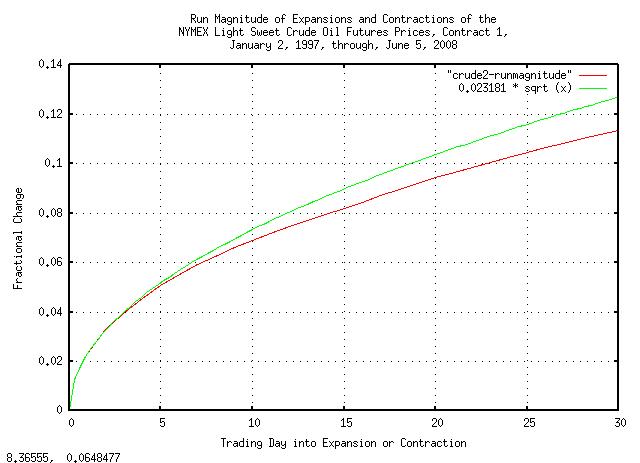
tsmath -l crude2.txt | tslsq -o | tsrunmagnitude -r 0.498672 > crude2-runmagnitude
|
Figure XXIII is a plot of the magnitude of the expansions and contractions of the NYMEX light sweet crude oil futures prices, contract 1, January 2, 1997, through, June 5, 2008. And, again, notice how well the the empirical data matches the theoretical data.
Again, notice the efficiency of the crude oil market-the root of
the magnitude of the expansions and contractions is
0.498672, very close to the
theoretical value of 0.5, (for
example, the DJIA runs about
0.56.)
However, note how fast the bubble has increased-its about
146 days old, and the standard deviation at 146 days would be a factor
of 0.023181 * sqrt (146) = 28%,
meaning the current bubble is a 55 / 28 =
1.96, (since it has increased about 55% in the
146 days,) or about a 2 sigma
occurrence, and there is about 2.2% chance of that happening, (and,
also, about a 2.2% chance of it getting much worse, before it gets
better.)
History of U.S. Bank Failures offers some interesting comments on US FDIC bank failures, and references the FDIC's the Closings and Assistance Transactions, 1934-2007. The FDIC's Institution Directory lists the current 8,417 institutions, of which 88.1% are profitable.
The best methodology would be to analyze the number of FDIC insured banks per year, (as a
high entropy geometric
progression,) but the data is not available, so only the failures
will be analyzed, (from Closings
and Assistance Transactions, 1934-2007, using a text editor to
fabricate the time
series, HSOB.txt,) as a
simple arithmetic progression, Brownian
Motion fractal.
tsrunlength HSOB.txt | tsmath -a 0.11624763874381928070 > HSOB.runlength+0.116
And graphing:
|
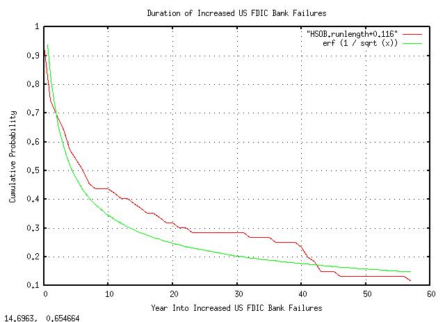
Figure XXIV is a plot of the duration of increased US FDIC bank failures. What the graph means is that at the beginning of a time interval of increasing bank failures, there is a 50% chance that the duration of increased bank failure rate will last at least 4 years, (i.e., 4 years is the median value,) and there is a 33% chance that it will last at least a decade.
    tsrootmean -p HSOB.txt
    0.459459        0.579007        0.679537        -0.050265t
    calc '(0.579007 + 0.679537) / 2'
    0.629272
    tsrunmagnitude -r 0.629272 HSOB.txt > HSOB.runmagnitude
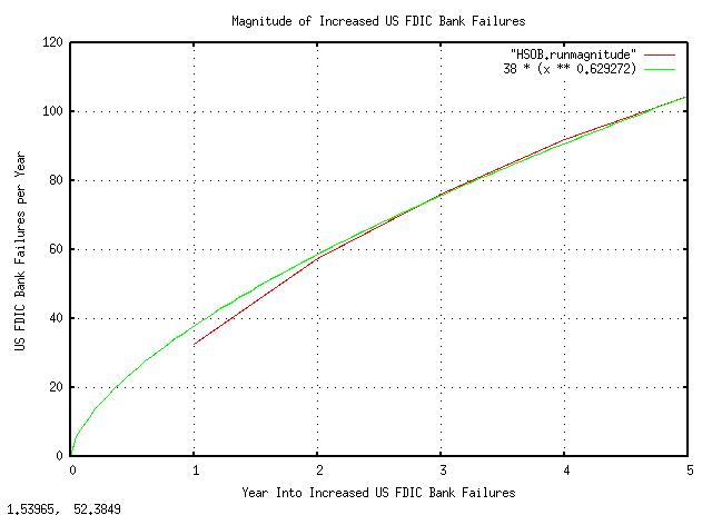
|
Figure XXV is a plot of the US FDIC bank failure rate in an interval
of increased failures. What the graph means is that there is a one standard
deviation, about 84%, that the number of bank failures in year 4
will be less than about 90, and a 16% chance, more. Note that there is
a 63% chance of what happened in the previous year, repeating in the
next year, and the standard
deviation = sqrt (variance)
is 38 failed banks per year.
    tsderivative HSOB.txt | tsnormal -t > HSOB.distribution
    tsderivative HSOB.txt | tsnormal -s 5 -t -f > HSOB.frequency
    tsderivative HSOB.txt | tsnormal -s 13 -t -f > HSOB.frequency
    tsderivative HSOB.txt | tsnormal -s 23 -t -f > HSOB.frequency
    tsderivative HSOB.txt | tsnormal -t -f > HSOB.frequency
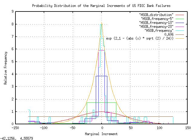
|
Figure XXVI is a plot of the probability distribution of the marginal increments of US FDIC bank failures. (The data set had
only 74 data points-which is inadequate for meaningful analysis-and
the graph was made by varying the size of the "buckets" in each
frequency distribution computation.) Note the Laplacian
distribution, meaning that banks fail randomly, and there is an
equal probability of a failure in any time interval. The
sqrt (variance),
computed by this method is 24 failed banks per year, (as opposed to 38
in the preceding graph.)
    tsderivative HSOB.txt | tsrms -p
    42.249747
Averaging the three values, (24, 38, 42,) of the sqrt
(variance)
= root-mean-square,
(rms,) gives the metric of the risk of bank failures at 35
per year. (Note that this is not the average failures per
year. It is a metric of the dispersion around the average, which is a
Laplacian
distribution, with fat tails, although some have
speculated that it is a Cauchy
Distribution.)
The beginning of the "great recession" brought on by housing asset value deflation, was forecast in Appendix VIII, Housing/Asset Prices, Sunnyvale, California, based on data from 1975 through 2007, by which time we were certain that a housing "bubble" crisis was inevitable.
The marginal increments of housing prices is simply the fractional change from one year to the next, i.e., subtract last year's price from the current year's price, and divide that by last year's price, (perhaps in a spreadsheet.) Do so for each year in the history, (since 1975 in this case.)
The sum of the marginal increments, divided by the number of years
is the average, (mean,) fractional growth of the house's value, (a
metric of the asset value's gain.) Call this value
avg, which is 0.082003 from the current
Office of Federal Housing Enterprise
Oversight data.
The square root of the sum of the squares of the marginal
increments, divided by the number of years is the variance of the
growth of the house's value, (the root-mean-square of the marginal
increments is a metric of the asset value's risk.) Call this value
rms, which is 0.136603 from the current
Office of Federal Housing Enterprise
Oversight data.
What this means is the average annual gain in value is about 8.2%
and the variance of the gain is 13.6%, meaning 8.2% +/- 13.6% gain for
68% of the years in the data, (because that's what variance means: 16%
of the years would have more than 8.2 + 13.6 =
21.8% gain, and 16% would have less than
8.2 - 13.6 = -5.4% gain, centered around
8.2% gain; a normal bell curve scenario, with the median, or center,
offset of 8.2%.)
(The following equations were derived in Quantitative Analysis of Non-Linear High Entropy Economic Systems I.)
What's the probability of a gain in any year, (Equation (1.24))?
        avg
        --- + 1
        rms
    P = ------- = 0.8001
           2
or about 80% of the years will have a gain in housing prices, and 20% will not.
Note that the average gain, avg, is
not really the long term gain to be expected!!! For that, (Equation
(1.20)):
                 P           1 - P
    G = (1 + rms) * (1 - rms)      = 1.076
for an annual gain of G = 7.6%.
So, how is that used to determine optimal leveraging to purchase a house? (Equation (1.18)):
f = (2 * P) - 1 = 0.6002
Or, considering it gambling, (its a worthwhile game, since one has
more than a 50/50 chance of winning,) one should wager f
= 60% of one's capital on each iteration of the game,
i.e., the down payment for the first year.)
But f, the variance of the marginal
increments, is only 13.6603%, which is too small, (i.e., no where near
60%.) This is where the engineering comes in. The question to ask is
what value of loan, and, initial down payment, will make the variance
of the down payment, (plus the increase in value of the house,) such
that the annual gain of the initial down payment is maximum and
optimized such that the risk is simultaneously minimized?
All I'm doing here is making the down payment work for me, maximally, and optimally, (less down, or more down, would give me less gain, in the long run,) with minimum risk to my down payment, (less down, or more down, would increase my chances of going bust, sometime in the future of the loan,) i.e., what we want to do is maximize the gain, and, simultaneously, minimize the risk.
LetX be the fraction of the total price
of the house that will be "owned" by the bank, and
V be the total price of the house, so
(1 - X) * V is my down payment, and
V * X is the amount of the loan. I have
a variance on the total value of the house of 0.136603, and need
0.6002:
    0.136603 * V
    ------------ = 0.6002
       V - X
And solving for X:
    0.136603 * V = (0.6002 * V) - (0.6002 * X)

    X = V * (1 - (0.136603 / 0.6002))

    X = 0.772404 * V
Or, the loan will be for about 77.2% of the house's value, and the down payment will be 22.8%.
Now, look at the gain in the principle value, (i.e., the down payment,) the first year (Equation (1.20)):
                 P           1 - P
    G = (1 + rms) * (1 - rms)      = 1.212741
Or, the expected return on investment, ROI, on the down payment to buy the house would be about 21% the first year.
Which is respectable. But it gets better.
Suppose the buyer of the house did so at the peak of the housing "bubble" in Q1 of 2006, with 22.8% down. Would the buyer be "underwater"?
The answer is that the vast majority would not have gone "underwater," and the "great recession" would have been avoided. The average buyer would not have much equity left, but would never have been "underwater," (and would have gained 6% back since Q4 of last year, 2010, when it bottomed, and would expect to make the down payment back in total within 4 years, or so.)
So, what's the moral?
Monetary policy to enhance prosperity by regulators allowing 1% down mortgage loans, with the risk distributed in credit default swaps was not very bright-it manufactured an unsustainable real estate "bubble," which would ultimately collapse into crisis, taking the money markets with it. Unsuspecting buyers inadvertently participating in the "bubble," and worse, refinancing to 1% equity to buy consumer items was not very bright, either. Once these happened, the "great recession" was an inevitability.
There is a similar story in the use of stock margins, (which were reduced to 10-15%, or so,) in 1999 and 1929, too.
Leveraging is a very important concept in finance, (in point of fact, it is one of the central concepts of mathematical finance,) when executed with skill. But too often, it is abused, and we seldom learn from the past.
For other comments about abusive leveraging and the "great recession", see: SFI Bulletin, 2009, vol.24, no.1 and read the article "Aftershocks of the Financial Earthquake," by John Whitfield, pp 32-36, and, "On Time and Risk," by Ole Peters, pp 36-41, which references the J. L. Kelly, Jr. 1956 paper, Bell System Technical Journal, "A New Interpretation of Information Rate." Note that the above methodology to find the optimal fraction of down payment for a real estate asset, (it works for buying equities with an optimal margin fraction, or optimal banking marginal reserves, too,) is nothing more than an application of the half century old Kelly paper-which introduced the so called "Kelly Criteria." For a non-mathematical treatment of the "Kelly Criteria," see the truly outstanding book by William Poundstone, "Fortune's Formula: The Untold Story of the Scientific Betting System that Beat the Casinos and Wall Street," Hill and Wang, New York, 2005, ISBN 0-8090-4637-7.
--

John Conover, john@email.johncon.com, http://www.johncon.com/