Quantitative Analysis of Non-Linear High Entropy Economic Systems VI

From: John Conover <john@email.johncon.com>
Subject: Quantitative Analysis of Non-Linear High Entropy Economic Systems VI
Date: 15 Oct 2004 19:27:49 -0000

Introduction

As mentioned in Section I, Section II, Section III, Section IV, Section V much of applied economics has to address non-linear high entropy systems-those systems characterized by random fluctuations over time-such as net wealth, equity prices, gross domestic product, industrial markets, etc.

The dynamics of non-linear high entropy systems are probabilistic in nature, and the understanding of the mathematics involved permits engineered solutions in the field of finance, such as development of strategies for portfolio growth optimization. However, leptokurtosis of the marginal increments of financial time series can lead to a very optimistic assessment of the actual long-term financial risk of an investment.

Note: the C source code to all programs used is available from the NtropiX Utilities page, or, the NdustriX Utilities page, and is distributed under License.

Methodology

As a demonstration of the effect of leptokurtosis in the marginal increments of a time series on the assessment of risk in an investment, the price history of the DJIA, (ticker symbol "^DJI",) was downloaded from Yahoo!'s Historical Prices database. The time series is the daily closes of the DJIA from January 2, 1900, through October 12, 2004, for 28,605 trading days. The csv format was converted to a Unix database format file, djia, using the csv2tsinvest program, from the NtropiX site.

From Section I, Important Formulas, Equation (1.24):



        avg
        --- + 1
        rms
    P = ------- ........................................(1.24)
           2

where avg and rms are the average and deviation of the marginal increments of the value of the DJIA, respectively, and P is the likelihood of an up movement in the value. From Equation (1.20):



                 P          (1 - P)
    g = (1 + rms)  (1 - rms)        ....................(1.20)

g is the average increase in the value of the DJIA per unity time, one trading day; for example, after n many days, an equity's value would have increased in value by a factor of g^n.

Using the tsfraction program on the time series, (presented in Figure I,) and piping the output to the tsavg and tsrms:



    tsfraction djia | tsavg -p
    0.000236

    tsfraction djia | tsrms -p
    0.011001

giving P = 0.51072629761 and g = 1.00017551026. To simulate this file, the tsinvestsim program from the from the NtropiX site was used, with an input file, tsinvestsim.djia.infile:



    djia, p = 0.51072629761, f = 0.011001, i = 68.13

and an output file, tsinvestsim.djia:



    tsinvestsim -n 10000 tsinvestsim.djia.infile 28605 | cut -f3 > tsinvestsim.djia

There is one other file that will be helpful in analyzing the leptokurtosis of the marginal increments of the DJIA-randomizing the marginal increments, and reconstructing a similar time series with the randomized increments. One method is to use the tsgaussian program to generate a time series of 28605 random numbers, and pasting the series into the djia file, sorting on the random numbers, and then removing the column of random numbers, which will resequence the marginal increments of the DJIA. The randomized marginal increments of the DJIA can be constructed into a fractal time series file, djia.random, using the tsunfraction program:



    tsgaussian 28605 > tsgaussian.tmp
    tsfraction djia > djia.tsfraction.tmp
    paste tsgaussian.tmp
    djia.tsfraction.tmp | sort -n | cut -f2 | tsunfraction -i 68.13 > djia.random

where the series of random numbers is tsgaussian.tmp, and the marginal increments of the DJIA is djia.tsfraction.tmp which are pasted together, in columns, with the Unix paste(1) command, and sorted with the sort(1) command, then the rearranged marginal increments removed with the cut(1) command, and finally, reassembled into a fractal time series using the tsunfraction command.

Figure I

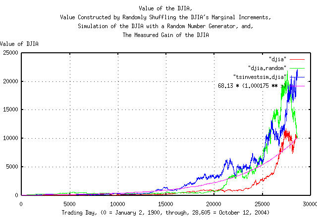
Figure I is a plot of the value of the DJIA's daily closes, from January 2, 1900, through, October 12, 2004, overlayed with the plot constructed by randomizing the marginal increments of the DJIA, and reconstructing a similar time series, followed by the plot of the simulation of the DJIA, constructed with a random number generator, and the measured gain of the DJIA.

The tsfraction and the tsnormal programs can be used to construct the frequency distributions of the marginal increments of the Brownian motion/random walk fractal equivalent of the DJIA time series, as described in Section II:



    tsfraction djia | tsnormal -t > djia.distribution
    tsfraction djia | tsnormal -t -f > djia.frequency
    tsfraction djia.random | tsnormal -t > djia.random.distribution
    tsfraction djia.random | tsnormal -t -f > djia.random.frequency
    tsfraction tsinvestsim.djia | tsnormal -t > tsinvestsim.djia.distribution
    tsfraction tsinvestsim.djia | tsnormal -t -f > tsinvestsim.djia.frequency

and plotting:

Figure II

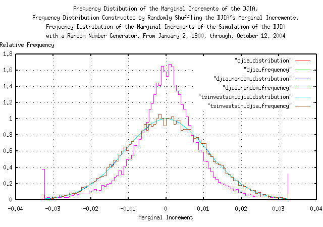
Figure II is a plot of the frequency distributions of the marginal increments of the DJIA's daily closes, from January 2, 1900, through, October 12, 2004, overlayed with the plot constructed by randomizing the marginal increments of the DJIA, and reconstructing a similar time series, followed by the plot of the simulation of the DJIA, constructed with a random number generator. The leptokurtosis of the DJIA's frequency distributions, of the DJIA, (the randomizing of the marginal increments had no effect on the leptokurtosis,) are visibly evident.

The simulation of the DJIA has a Hausdorff fractal dimension of 2, (by construction-the random number generator used in the tsinvestsim program produces a binomial distribution,) and the DJIA, (and the time series constructed by shuffling the DJIA's marginal increments,) have a fractal dimension that is somewhat less than 2.

The tsrunmagnitude can be used to measure the fractal dimension of the Brownian motion/random walk fractal equivalent of the DJIA time series, as described in Section II, with a shell script:



    #!/bin/sh
    R="0.500000"
    LASTR="1.000000"
    while [ "${R}" != "${LASTR}" ]
    do
        LASTR="${R}"
        echo "${R}"
        tsmath -l input | tslsq -o | tsrunmagnitude -r "${R}" > "input.tsrunmagnitude-r${R}"
        cut -f1 "input.tsrunmagnitude-r${R}" | tsmath -l > input.tsrunmagnitude.log.1
        cut -f2 "input.tsrunmagnitude-r${R}" | tsmath -l > input.tsrunmagnitude.log.2
        R=`paste input.tsrunmagnitude.log.1 input.tsrunmagnitude.log.2 | egrep '^[0-5]\.' | \
            tslsq -p | sed -e 's/^.*\+ //' -e 's/t$//'`
    done

The shell script iterates improvements in the accuracy of the estimate of the fractal dimension of the time series in file, input, starting with an initial guess of 0.5, (corresponding to a fractal dimension of 2, which represents a Gaussian/normal distribution of the marginal increments of the Brownian motion/random walk fractal equivalent of the time series.)

For the DJIA's time series file, djia, the iteration sequence is:

Meaning that the fractal dimension of the Brownian motion/random walk equivalent of the DJIA's time series is 1 / 0.542043 = 1.84487208579. For the time series made by shuffling the DJIA's marginal increments in file, djia.random:

Or the fractal dimension of the Brownian motion/random walk equivalent of the time series made by shuffling the DJIA's marginal increments is 1 / 0.484637 = 2.0634000293. Lastly, for the time series, tsinvestsim.djia for the simulation of the DJIA, constructed with a random number generator:

Which has a fractal dimension of the Brownian motion/random walk equivalent of the simulation of the DJIA, constructed with a random number generator of 1 / 0.493159 = 2.02774358777.

And plotting:

Figure III

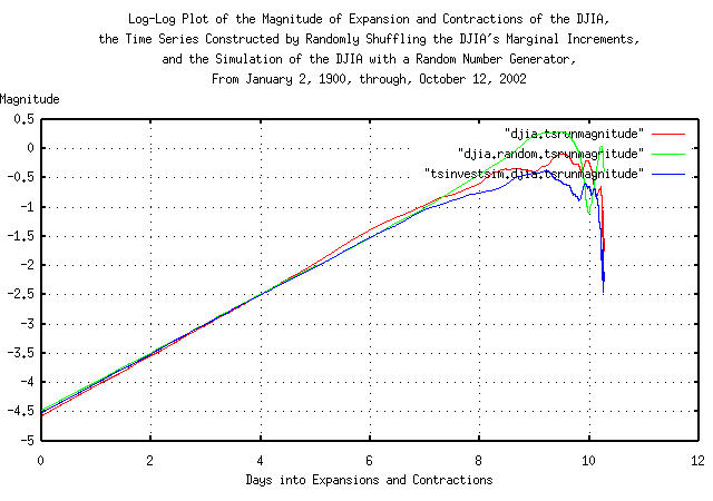
Figure III is a log-log plot of the magnitude of the expansions and contractions of the DJIA's daily closes, from January 2, 1900, through, October 12, 2004, overlayed with the plot constructed by randomizing the marginal increments of the DJIA, and reconstructing a similar time series, followed by the plot of the simulation of the DJIA, constructed with a random number generator. Its convenient since the slope of the lines is the reciprocal of the fractal dimension of the three time series.

As a side bar, a Brownian motion time series would have random increments that sum together-making expansions and contractions that have a magnitude proportional to the square root of time-the process would operate as:



               2    2    2
          V      = V  + R  ..............................(6.1)
           n + 1    n    n

where the next value, squared, is equal to the previous value, squared, plus the value of a random number squared, (i.e., its a root-mean-square operation.) But this is true, if and only if, the random number has a Gaussian/normal distribution. The Gaussian/normal distribution is only one of a family-the family of interest in non-linear high entropy economic systems usually have exponents that range from 1, (a Cauchy distribution, see: Appendix I,) to 2, (a Gaussian/normal distribution.) In general, for the family of fractals:



               k    k    k
          V      = V  + R  ..............................(6.2)
           n + 1    n    n

where 1 / k is the slope of the curve in Figure III.

The exponent k determines which mathematics to use when summing random numbers to make a time series. The exponent k is the fractal dimension of the time series. For a simple Brownian motion type of time series, k = 2. At the other extreme, for a time series with Cauchy distributed marginal increments, k = 1, meaning the increments add linearly instead of as root-mean-square for Gaussian/normal distributed marginal increments. Most often the fractal dimension lies between these two values.

Of interest is that as k decreases from 2, (which is the case of the ubiquitous Gaussian/normal distributed increments,) to 1, adding N independent Cauchy distributed variables together results in a Cauchy variable that has the same distribution as the originals-there is no advantage to averaging Cauchy variables.

Figure III is worthy of attention. Note that the fractal dimension of the Brownian motion/random walk equivalent of the simulation of the DJIA is not constant-the graph is steeper at about e^0, about 3 trading days, and at about e^5.5, 253 trading days. These are market inefficiencies-everyone does not respond to market information instantaneously; it takes several days for the market to adjust to new information. And in the latter case, there is correlation between 4'th calendar quarters, (about 253 trading days,) of years-this is a structural inefficiency; the tax code makes it advantageous to dump under performing equities from portfolios, driving the market to a lower level-supply exceeding demand:



    egrep '^[0]\.' djia.tsrunmagnitude | tslsq -p
    -4.570576 + 0.526275t

    egrep '^[1-4]\.' djia.tsrunmagnitude | tslsq -p
    -4.572585 + 0.519285t

    egrep '^[5]\.' djia.tsrunmagnitude | tslsq -p
    -4.824752 + 0.573925t

and in between, around e^3, or 20-60 trading days, the fractal dimension is almost equal simple Brownian motion. The numbers indicate that there is about a 53% chance that what happens one day, will happen the next, too; and in calendar quarter 4, there is a 57% chance of increased volatility, (usually, a down side.)

Of further interest, note that the Brownian motion/random walk equivalent of the time series made by shuffling the DJIA's marginal increments does not have a larger slope in Figure III, even though the leptokurtosis in Figure II, is unaffected.

The best fit standard deviation for the expansion and contractions of the Brownian motion/random walk equivalent of the time series is:



    paste djia.tsrunmagnitude.log.1 djia.tsrunmagnitude.log.2 > \
        djia.tsrunmagnitude
    egrep '^[0-5]\.' djia.tsrunmagnitude | tslsq -p
    -4.650909 + 0.542043t

    paste djia.random.tsrunmagnitude.log.1 djia.random.tsrunmagnitude.log.2 > \
        djia.random.tsrunmagnitude
    egrep '^[0-5]\.' djia.random.tsrunmagnitude tslsq -p
    -4.437246 + 0.484637t

    paste tsinvestsim.djia.tsrunmagnitude.log.1 tsinvestsim.djia.tsrunmagnitude.log.2 > \
        tsinvestsim.djia.tsrunmagnitude
    egrep '^[0-5]\.' tsinvestsim.djia.tsrunmagnitude tslsq -p
    -4.481453 + 0.493159t

The formula for the standard deviation of the magnitude of the expansions and contractions of the Brownian motion/random walk equivalent of the time series for the DJIA is e^-4.650909 * (x^0.542043) = 0.00955291438 * (x^0.542043), and for the time series made by shuffling the DJIA's marginal increments, e^-4.437246 * (x^0.484637) = 0.0118284693 * (x^0.484637), and for the simulation of the DJIA made with a random number generator, e^-4.481453 * (x^0.493159) = 0.0113169577 * (x^0.493159).

Plotting:

Figure IV

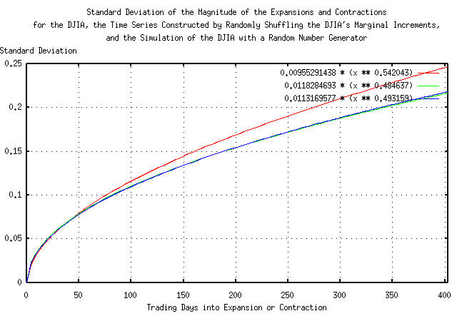
Figure IV presents the standard deviation of the magnitude of the expansions and contractions of the Brownian motion/random walk equivalent of the time series for the DJIA, 0.00955291438 * (x ** 0.542043), the time series made by shuffling the DJIA's marginal increments, 0.0118284693 * (x ** 0.484637), and the simulation of the DJIA made with a random number generator, 0.0113169577 * (x ** 0.493159).

Note that for time intervals less than about 20 trading days, (about a calendar month,) there is little or no difference between the three graphs-the leptokurtosis has little effect. However, at longer time intervals, the actual DJIA diverges from the other two graphs.

As a side bar, the graphs in Figure IV represent the way the fractals operate-the way they add random numbers together as time goes on. In the bottom two graphs, the mechanism is very close to a root-mean-square operation.

Not so for the DJIA-instead of a square root summing process, 0.5000000, it is a summing process of a 0.542043 operation-and those two numbers are metrics of risk.

The formula for the way a Gaussian/random process works is:



               2    2    2
          V      = V  + R  ..............................(6.1)
           n + 1    n    n

while for the DJIA, (1 / 0.542043 = 1.8448720579, about 1.8):



               1.8    1.8    1.8
          V        = V    + R    ........................(6.3)
           n + 1      n      n

So, (using ((0.00955291438 * (t^0.542043)) / (0.011001 * (t^0.5)) - 1.0), where t is trading days,) at:

One day, the error would be -13.163218071%
One trading week of 5 days, the error would be -7.083997602%
One trading month of 20 days, the error would be -1.507553612%
One trading year of 253 days, the error would be 9.581720969%
One trading decade of 2530 days, the error would be 20.720525342%

Note that for an analysis of the DJIA with prediction times running less than about 20 days into the future using root-mean-square mathematics, the predicted risk is larger than it really is, and for more than about 20 days, the predicted risk is smaller.

The Hurst Exponent

Several alternative methods exist for finding the fractal dimension of a financial time series such as the discrete Fourier transform which is used in the tsdft program and the Hurst exponent as used in the tshurst program. Because of its ubiquitous usage, the Hurst exponent will be compared with the results from the tsrunmagnitude program, above.



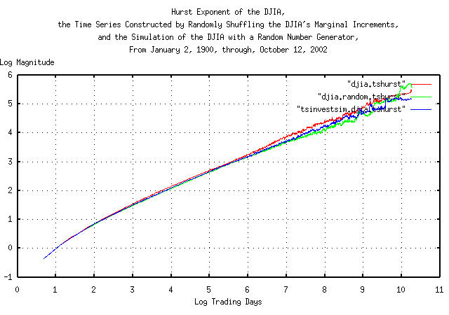
    tsmath -l djia | tslsq -o | tshurst > djia.tshurst
    egrep '^[5]\.' djia.tshurst | tslsq -p
    -0.058516 + 0.549039t

    tsmath -l djia.random | tslsq -o | tshurst > djia.random.tshurst
    egrep '^[5]\.' djia.random.tshurst | tslsq -p
    0.034777 + 0.522176t

    tsmath -l tsinvestsim.djia | tslsq -o | tshurst > tsinvestsim.djia.tshurst
    egrep '^[5]\.' tsinvestsim.djia.tshurst | tslsq -p
    0.127771 + 0.508337t

Plotting:

Figure V

Figure V presents the Hurst exponent of the Brownian motion/random walk equivalent of the time series for the DJIA, the time series made by shuffling the DJIA's marginal increments, and the simulation of the DJIA made with a random number generator. The slope of the graphs is the Hurst exponent-and that presents a problem with a 28,605 record time series; the Hurst methodology uses root-mean-square mathematics and subtracts the mean of the intervals used to calculate the fractal dimension which gives poor accuracy below about e^5 = 148 days, and data set size restrictions limit the accuracy above about 148 days. In no way, however, does this detract from the significant contributions Hurst made to fractal analysis-the methodology has been a standard for half a century.

The Hurst methodology does agree fairly well with the iterated methodology outlined above using the tsrunmagnitude program in Figure III but without adequate accuracy in the near term of a few trading days.

Interestingly, the Hurst methodology does detect the short term and annual market inefficiencies of the DJIA.

A note about definitions. A classical ordinary Brownian motion fractal has a Hurst exponent, H = 0.5, and a Gaussian/normal distribution of the marginal increments. A fractional Brownian motion fractal has a Hurst exponent 0.0 < H < 1.0, and also has a Gaussian/normal distribution of the marginal increments. Ordinary Brownian motion fractals are a subset of the family of fractional Brownian motion fractals. However, ordinary Brownian motion fractals have statistical independence of the marginal increments, which is not so for fractional Brownian motion fractals. The marginal increments of a fractional Brownian motion fractals are not statistically independent-even though they have a Gaussian/normal distribution.

Leptokurtosis is not associated with either ordinary or fractional Brownian motion fractals-it is a different mechanism, altogether, that is associated with a non-linearity, (like the tan () operator/function in the Cauchy distribution,) in the fractal's random process.

Both the effects of leptokurtosis, and the statistical dependence of the marginal increments of fractional Brownian motion fractals are detected by the Hurst methodology-but the methodology can not distinguish between the two, (or combination thereof.)

Statistical dependence of the marginal increments of a fractional Brownian motion fractal is exploitable as a regressive forecasting mechanism in financial time series-leptokurtosis in the distribution of the marginal increments of a fractal is not.

As a side bar, randomizing the marginal increments of a fractal time series, and reconstructing a fractal from the randomized marginal increments, destroys any statistical dependence of the fractal's marginal increments-without changing the distribution of the marginal increments. The distribution is the same in the original and randomized fractals.

The difference between the Hurst exponents for the djia and djia.random files in Figure V, above, is, (approximately,) created by the statistical dependence of the marginal increments in the djia file.

Formally, the term leptokurtosis means a centrally peaked distribution of a fractal's marginal increments that has fat tails, like the DJIA in figure Figure II. However, more commonly, it refers to any distribution that deviates from a statistically independent Gaussian/normal distribution-which is often used in modeling complex distributions as a mathematical expediency.

The centrally peaked section of a leptokurtic distribution means there are too many small increments to be accounted for, and usually have little significance on the assessment of risk. However, the fat tails are far more problematical-they mean there are too many very large increments to be accounted for and they occur too frequently-and are often modeled with Cauchy-like distributions.

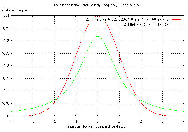
Appendix I, The Gaussian/Normal and Cauchy Frequency Distributions

Fractal dimensions lie between zero and two, (dimensions greater than two have negative probabilities,) and financial time series of non-linear high entropy economic systems usually lie between one and two; a fractal dimension of two means the fluctuations in the system's process is characterized by a Gaussian/normal distribution, and at the other extreme, a fractal dimension of one means the fluctuations in the system's process is characterized by a Cauchy distribution. The fractal dimension is a metric of how rough the system's responses are; a Gaussian/normal distribution is the ubiquitous bell shaped curve with small tails, while a Cauchy distribution has fat tails showing that extreme jumps in the system characteristics are much more common.

The formula for the Gaussian/normal distribution is :



    f(x) = (1 / sqrt (2 * pi)) * e^(- (x^2) / 2) ........(6.4)

And for a Cauchy distribution:



                  1
    f(x) = ---------------- .............................(6.5)
           pi * (1 + (x^2))

And Plotting:

Figure V

Figure V presents the Gaussian/normal and Cauchy frequency distributions. Most financial time series of non-linear high entropy economic systems usually have frequency distributions that lie between the Gaussian/normal and Cauchy frequency distributions-with most being closer to a Gaussian/normal distribution; enough so that it is often used as a mathematical expediency in analysis-the assumed mathematics to use for a Gaussian/normal frequency distribution is root-mean-square, i.e., when adding variables, they are squared, added together, and then the square root taken of the sum.

It is very easy to construct a time series that has a Cauchy frequency distribution using a computer's uniform random number generator on the interval [0,1]:



    C = tan (pi * (0.5 - U))

which produces a Cauchy variable, C from a uniform variable, U. This is the mechanism used in the tscauchy program. Making two time series, one with variables that have a Gaussian/normal frequency distribution, and the other with variables that have a Cauchy distribution:



    tsgaussian 100000 > gaussian
    tscauchy 100000 > cauchy

and analyzing as was done in Figure III, above:



    tsintegrate gaussian | tsrunmagnitude -r 0.500000 > tsgaussian.tsrunmagnitude-r0.500000
    cut -f1 tsgaussian.tsrunmagnitude-r0.500000 | tsmath -l > tsgaussian.tsrunmagnitude.log.1
    cut -f2 tsgaussian.tsrunmagnitude-r0.500000 | tsmath -l > tsgaussian.tsrunmagnitude.log.2
    paste tsgaussian.tsrunmagnitude.log.1 tsgaussian.tsrunmagnitude.log.2 > \
        tsgaussian.tsrunmagnitude
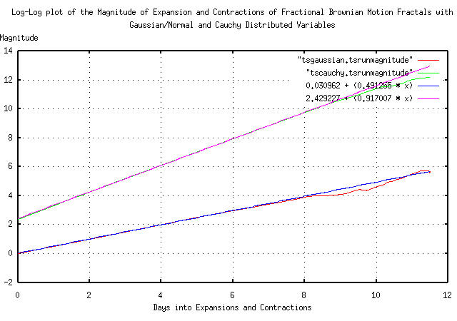
    egrep '^[0-5]\.' tsgaussian.tsrunmagnitude | tslsq -p
    0.030962 + 0.491255t

    tsintegrate cauchy | tsrunmagnitude -r 1.000000 > tscauchy.tsrunmagnitude-r1.000000
    cut -f1 tscauchy.tsrunmagnitude-r1.000000 | tsmath -l > tscauchy.tsrunmagnitude.log.1
    cut -f2 tscauchy.tsrunmagnitude-r1.000000 | tsmath -l > tscauchy.tsrunmagnitude.log.2
    paste tscauchy.tsrunmagnitude.log.1 tscauchy.tsrunmagnitude.log.2 > \
        tscauchy.tsrunmagnitude
    egrep '^[0-5]\.' tscauchy.tsrunmagnitude | tslsq -p
    2.429227 + 0.917007t

which is very close to the theoretical values of 0.5 for the Gaussian/normal distribution, and 1.0 for the Cauchy.

And Plotting:

Figure VI

Figure VI is a log-log plot of the magnitude of the expansions and contractions of a Brownian motion time series with a Gaussian/normal frequency distributed variable, and a time series with a Cauchy frequency distributed variable. The fractal dimension of each is the reciprocal of the slope of the two graphs. The fractal dimension of the Gaussian/normal distribution is 1 / 0.5 = 2 and for the Cauchy, 1 / 1 = 1 meaning that the formula, i.e., the mathematics, for adding Gaussian/normal frequency distributed variables, VN, is V1^2 + V2^2 ... and Cauchy frequency distributed variables, V1 + V2 ....

Note the difficulty of working with Cauchy frequency distributed variables-the graph in Figure VI should intersect the y-axis at ln (2) = 0.693 ..., but since the distribution of N many identically distributed Cauchy variables is the same as the originals, averaging, (as in integrating or summing, and dividing by N,) does not improve the estimate. (Why should the graph intersect the y-axis at 2? Because the effective value of the Cauchy variables is the interquartile range, which is the difference between the two x values for which the integral of Equation ( 6.5) equal 1 / 4 and 3 / 4-which is 2 for Equation ( 6.5).)

As a side bar, the Cauchy and Gaussian/normal distributions are at opposite ends of the family of Levy-Stable distributions. If the marginal increments of a time series has a Gaussian/normal distribution, then they add root-mean-square. Using the file djia as an example:



          tsfraction djia | tsrms -p
          0.011001

where the root-mean-square of the marginal increments is the metric of risk. But the equivalent metric of risk for Cauchy distributions is the interquartile range, (i.e., the values at 25% and 75% of the integral of the distribution):



          tsfraction djia | sed 's/[0-9][0-9]$//' | sort -n | \
              tscount | cut -f1 > tmp.1
          tsfraction djia | sed 's/[0-9][0-9]$//' | sort -n | \
              tscount | cut -f2 > tmp.2

          paste tmp.2 tmp.1 | tsintegrate -t | tail -1
          0.1534  28604.000000

          paste tmp.2 tmp.1 | tsmath -t -d 28604 | \
              tsintegrate -t | egrep '0\.25'
          -0.0045 0.252060
          -0.0044 0.255766

          paste tmp.2 tmp.1 | tsmath -t -d 28604 | \
              tsintegrate -t | egrep '0\.75'
          0.0053  0.753179
          0.0054  0.757095

or the interquartile range is 0.0045 + 0.0053 = 0.0098, which is the metric of risk assuming the DJIA has a Cauchy distribution of its marginal increments.

If the marginal increments of the DJIA have a distribution from the Levy-Stable family, then the metric of risk lies between 0.011001 and 0.0098, which differ by a factor of 0.011001 / 0.0098 = 1.12255102041, or about 10%; the actual value of risk would be between these two numbers.

Note that Generalized Gaussian Density Model techniques do exist for measuring the parameters of the distribution of the marginal increments of financial time series, (the standard deviation of the density is, of course, the metric of risk.)

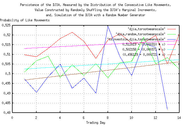
Appendix II, The Frequency Distribution of Like Consecutive Movements

The number of consecutive like movements of the marginal increments of a time series can be tallied, at different scales, and the resultant value of the frequency distribution of like movements calculated-for example, a simple random walk fractal with Gaussian/normal distributed increments would be the combinatorial probabilities, 0.5, 0.25, 0.125, 0.625 ...

The technique is mentioned only in passing. It requires a substantial amount of data for any reasonable accuracy, but has the advantage that it is applicable to Kalman filter techniques, where the initial assessment of persistence in the time series is quite rough but as more data is acquired, the accuracy increases. It is not an iterated technique.



    tsmath -l input | tslsq -o | tsrootmeanscale | cut -f1,3 > djia.tsrootmeanscale
    tslsq -p djia.tsrootmeanscale
    0.512819 + 0.000310t

    tsmath -l input | tslsq -o | tsrootmeanscale | cut -f1,3 > djia.random.tsrootmeanscale
    tslsq -p djia.random.tsrootmeanscale
    0.512819 + 0.000310t

    tsmath -l input | tslsq -o | tsrootmeanscale | cut -f1,3 > tsinvestsim.djia.tsrootmeanscale
    tslsq -p tsinvestsim.djia.tsrootmeanscale
    0.512819 + 0.000310t

And Plotting:

Figure VI

Figure VI is a plot of the least squares fit of the relative frequency of like movements in the marginal increments of the DJIA, from January 2, 1900, through October 12, 2004, for 28,605 trading days. Notice how rough the data is, even with moderate data set sizes. The technique is only useful for short term forecasting of a few trading days. Statistical estimation of the accuracy of the technique is challenging, but the methodology outlined in the tsshannoneffective program is applicable.

Appendix III, GE Equity Price

As a demonstration of the effect of leptokurtosis in the marginal increments of a time series on the assessment of risk in an investment, the price history of GE's equity price, (ticker symbol "GE",) was downloaded from Yahoo!'s Historical Prices database. The time series is the daily closes of the GE from March 26, 1991, through October 18, 2004, for 3,420 trading days. The csv format was converted to a Unix database format file, ge, using the csv2tsinvest program, from the NtropiX site.

Using the tsfraction program on the data in Figure IX, and piping the output to the tsavg and tsrms:



    tsfraction ge | tsavg -p
    0.001191

    tsfraction ge | ge -p
    0.018141

giving P = 0.532826195 and g = 1.00102708274. To simulate this file, the tsinvestsim program from the from the NtropiX site was used, with an input file, tsinvestsim.ge.infile:



    ge, p = 0.532826195, f = 0.018141, i = 1.00

and an output file, tsinvestsim.ge:



    tsinvestsim -n 10000 tsinvestsim.ge.infile 28605 | cut -f3 > tsinvestsim.ge

And Plotting:

Figure IX

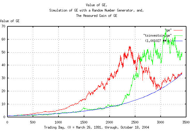
Figure IX is a plot of the value of GE's daily closes, from March 26, 1991, through, October 18, 2004, overlayed with the plot constructed with a random number generator, and the measured gain of the GE's equity price.

The tsfraction and the The tsnormal programs can be used to construct the frequency distributions of the marginal increments of the Brownian motion/random walk fractal equivalent of the GE's equity price time series, as described in Section II:



    tsfraction ge | tsnormal -t > ge.distribution
    tsfraction ge | tsnormal -t -f > ge.frequency
    tsfraction tsinvestsim.ge | tsnormal -t > tsinvestsim.ge.distribution
    tsfraction tsinvestsim.ge | tsnormal -t -f > tsinvestsim.ge.frequency

And Plotting:

Figure X

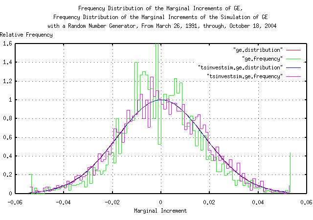
Figure X is a plot of the frequency distributions of the marginal increments of GE's equity price daily closes, from March 26, 1991, through, October 18, 2004, overlayed with the plot of the simulation of the GE's equity price, constructed with a random number generator.

The tsrunmagnitude can be used to measure the fractal dimension of the Brownian motion/random walk fractal equivalent of GE's equity price time series, as described in Section II, with a shell script:



    #!/bin/sh
    R="0.500000"
    LASTR="1.000000"
    while [ "${R}" != "${LASTR}" ]
    do
        LASTR="${R}"
        echo "${R}"
        tsmath -l input | tslsq -o | tsrunmagnitude -r "${R}" > "input.tsrunmagnitude-r${R}"
        cut -f1 "input.tsrunmagnitude-r${R}" | tsmath -l > input.tsrunmagnitude.log.1
        cut -f2 "input.tsrunmagnitude-r${R}" | tsmath -l > input.tsrunmagnitude.log.2
        R=`paste input.tsrunmagnitude.log.1 input.tsrunmagnitude.log.2 | \
            egrep '^[0-5]\.' | tslsq -p | sed -e 's/^.*\+ //' -e 's/t$//'`
    done

For GE's equity price time series file, ge, the iteration sequence is:

Meaning that the fractal dimension of the Brownian motion/random walk equivalent of the GE's equity price time series is 1 / 0.591312 = 1.69115458506. For the simulation of GE's equity price constructed with a random number generator:



    0.500000
    0.498553
    0.497645

Which has a fractal dimension of the Brownian motion/random walk equivalent of the simulation of the GE's equity price, constructed with a random number generator of 1 / 0.497645 = 2.00946457816.

And Plotting:

Figure XI

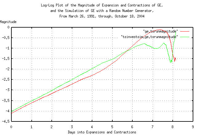
Figure XI is a log-log plot of the magnitude of the expansions and contractions of the daily close of the GE's equity price, from March 26, 1991, through, October 18, 2004, overlayed with the plot of the simulation of GE's equity price, constructed with a random number generator. The slope of the lines is the reciprocal of the fractal dimension of both time series.

The best fit standard deviation for the expansion and contractions of the Brownian motion/random walk equivalent of the time series is:



    paste ge.tsrunmagnitude.log.1 ge.tsrunmagnitude.log.2 > ge.tsrunmagnitude
    egrep '^[0-5]\.' ge.tsrunmagnitude | tslsq -p
    -4.571974 + 0.591312t

    paste tsinvestsim.ge.tsrunmagnitude.log.1 tsinvestsim.ge.tsrunmagnitude.log.2 > \
        tsinvestsim.ge.tsrunmagnitude
    egrep '^[0-5]\.' tsinvestsim.ge.tsrunmagnitude | tslsq -p
    -3.979742 + 0.497645t

The formula for the standard deviation of the magnitude of the expansions and contractions of the Brownian motion/random walk equivalent of GE's equity price time series is e^-4.571974 * (x^0.591312) = 0.010337533 * (x^0.591312), and for the simulation of GE's equity price made with a random number generator, e^-3.979742 * (x^0.497645) = 0.0186904609 * (x^0.497645).

And Plotting:

Figure XII

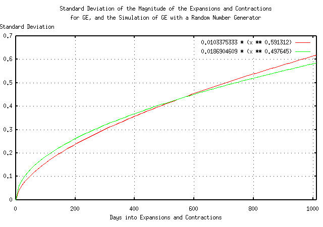
Figure XII presents the standard deviation of the magnitude of the expansions and contractions of the Brownian motion/random walk equivalent of the time series for GE's equity price

Note that for time intervals less than about 500 trading days, (about two calendar years,) there is little or no difference between the two graphs-the leptokurtosis has little effect. However, at longer time intervals, the actual GE equity price diverges.

Appendix IV, Leptokutosis of the DJIA

It would be desirable to decide whether the DJIA's marginal increments have a frequency distribution that is closer to Gaussian/normal or Cauchy distribution. The Gaussian/normal least squares best fit of the DJIA's marginal increments is shown in Figure II. If the marginal increments have a Cauchy distribution, then simply taking the arc tangent of the increments should reveal a simpler distribution, (see: Appendix I for the reasoning,) after appropriate rescaling.



    tsfraction djia | tsavg -p
    0.000236

    tsfraction djia | tsrms -p
    0.011001

There are 13 marginal increments in the DJIA, out of a total of 28606, that are larger than 0.1, or 13 / 28606 = 0.000454450115, which is about 3.32 standard deviations, or the singularity of the tangent function, at pi / 2, should be near 3.32 * 0.011001 = 0.03652332, or the scaling factor would be (pi / 2) / 0.03652332, which is about 43.

The tangent function has little effect for small values-those well below 3 standard deviations-so choosing 2 standard deviations, the amplitude scaling factor would be (2 * 0.011001) / tan (43 * 0.022002), which is about 0.016.

So, the formula for the leptokurtic non-linearity would be * 0.016 tan (43 * x).

The inverse formula for the leptokurtic non-linearity would be atan ((0.016 * tan (43 * x)) / 0.016) / 43 which would be about 0.023 atan (62.5 * x).

All that is necessary is to make the marginal increments of the DJIA, (using the tsfraction program,) and subtract the mean, (using the tsmath program,) and format each record, (using sed,) to make a stream of calculations for the calc program-which takes the arc tangent of each record. The frequency distribution of the marginal increments of the DJIA, after having the leptokurtic non-linearity removed will be calculated by the tsnormal program.



    tsfraction djia | tsmath -s 0.000236 | sed -e 's/^/0.023 * atan (62.5 * /' -e 's/$/)/' | \
        calc | sed 's/~//' | tsnormal -t > djia.atan.distribution
    tsfraction djia | tsmath -s 0.000236 | sed -e 's/^/0.023 * atan (62.5 * /' -e 's/$/)/' | \
        calc | sed 's/~//' | tsnormal -t -f > djia.atan.frequency

And Plotting:

Figure XIII

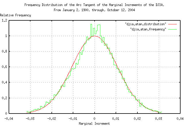
Figure XIII is a plot of the frequency distribution of the marginal increments of the DJIA's daily closes from January 2, 1900, through, October 12, 2004, with the leptokurtic non-linearity removed under the assumption that the marginal increments have a Cauchy-like frequency distribution. It is an impressive graphic that demonstrates better accuracy than the assumption that the marginal increments of the DJIA have a Gaussian/normal distribution, as shown in Figure II.

Note the use of the term Cauchy-like frequency distribution. The Cauchy distribution is produced by the tangent of a uniform distribution, where Figure XIII was produced by the tangent of, apparently, a Gaussian/normal distribution; it is doubtful that the tangential singularities really exist, and the leptokurtic non-linearity is created by a complex distribution of risk aversion, on the down side, to large movements in the marginal increments of the time series-a psychological phenomena. A simple exponential may be a better model of the non-linearity. However, assuming a Cauchy distribution as a worst case assessment of risk does seem viable for daily financial time series-an almost certainly conservative methodology, i.e., using the interquartile range of the increments that add linearly, (instead of as root-mean-square for Gaussian/normal distributed marginal increments,) to gain insight into the horizon of applicability of root-mean-square methodologies.

As a side bar, why does the assumption that the marginal increments of the DJIA have a Gaussian/normal distribution work?

It is because, for the very small values, (like a few percent,) seen in the marginal increments of daily financial time series, tan (x) is approximately equal to x.

However, for larger values-like those in the tails of the distribution of the marginal increments-the leptokurtic non-linearity makes the assumption invalid.

As a concluding note, although a non-linear tangential/Cauchy risk function was used in this worst case analysis, similar arguments could be made for the use of the hyperbolic arc tangent, (which is similar,) as well as the Levy stable distributions-which are attractive since they are not symmetrical, and the distribution is skewed to the positive side, (which is apparent in Figure XIII, and would preclude the possibility/probability of an equity's value becoming negative, which symmetrical distributions do not, e.g., minimizing the probability of a negative marginal increment larger than unity, even though a positive increment larger than unity is permitted.) However, all of these distributions have means and variances that diverge to infinity leading to long term expansions and contractions in financial data with incorrect shapes, limiting their use to conservative worst case analysis, (for example, the distribution of the magnitude of expansions and contractions in financial data would be linear for Cauchy distributed marginal increments, and square root for the Gaussian/Normal distributed increments.)

Appendix V, Empirical methodology for the leptokutosis of the DJIA

Meticulous methodologies must be employed when predicting the probability of extremely rare catastrophic economic events. To illustrate the range of errors induced in long range economic forecasts, the 1929 "crash" of the DJIA will be analyzed using a purely empirical methodology, and then compared with the predictions presuming a Gaussian/normal and Cauchy frequency distribution of the daily closes of the DJIA's marginal increments. The empirical methodology will presume only that the DJIA time series is a geometrical progression-and there is ample theoretical and empirical data that it is-and the marginal increments have a Pareto-Levy stable frequency distribution. (The Gaussian/normal and Cauchy are the only Pareto-Levy frequency distributions with analytical solutions-meaning that, in general, empirical methodologies are all that is available for analysis.)

On September 3, 1929, the DJIA was at a record high of 381.17. It then deteriorated to 41.22, a low for the entire Twentieth Century, on July 8, 1932, a decline of 89.1859275%, in 843 trading days.

The empirical methodology:

Finding the median value of the fractional Brownian equivalent of the DJIA:



    tsmath -l djia1900-2004 | tslsq -p
    3.475236 + 0.000169t

in 843 days, the median value of the fractional Brownian equivalent of the DJIA's would be 0.000169 * 843 = 0.142467, so the actual decline would be 41.22 / (381.17 * 1.142467) = 94.655447% from its median value.

Iterating the tsrunmagnitude program to compute the root, (i.e., the reciprocal of the Hausdorff fractal dimension,) using the djiaroot script:



    djiaroot
    LSQ Approximation = -4.588093 + 0.537910t, Error = 0.03791
    LSQ Approximation = -4.645150 + 0.541671t, Error = 0.003761
    LSQ Approximation = -4.650391 + 0.542009t, Error = 0.000338
    Final LSQ Approximation -4.650391 + 0.542009t

Figure XIV

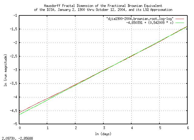
Figure XIV is a log-log plot of the final iteration of the tsrunmagnitude program in the djiaroot script, and its e^6 = 403 trading day LSQ best fit. The slope of the line is the root, i.e., the reciprocal of the Hausdorff fractal dimension of the fractional Brownian equivalent of the DJIA. The Hausdorff dimension specifies the math that is used in the fluctuation mechanism of the DJIA; A reciprocal of the Hausdorff dimension equal to 0.5 would mean a Gaussian/normal distribution of the marginal increments, and 1.0 would mean a Cauchy distribution. The DJIA's value lies in between these two values, and is 0.542009

Using e^-4.650391 = 0.00955786407 as the "deviation", (actually, the effective deviation-since the term is generally applied to Gaussian/normal frequency distributions,) and 0.542009 as the reciprocal of the Hausdorff fractal dimension, the deviation of the fractional Brownian equivalent of the DJIA from its median at 843 trading days would be

0.00955786407 * 843^0.542009 =
0.368286439

. 0.94655447 which would be

0.94655447 / 0.368286439 =
2.57015835981

deviations, which has a value of

0.00955786407 * 2.57015835981 =
0.0245652242

The cumulative distribution of the increments of the fractional Brownian equivalent of the DJIA can be calculated using the djiacumulativedistribution script, which produced the djia1900-2004.cumulative.distribution file, and is plotted in Figure XV.

Figure XV

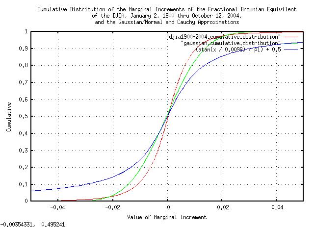
Figure XV is a plot of the cumulative distribution of the increments of the fractional Brownian equivalent of the DJIA contained in the djia1900-2004.cumulative.distribution file. The plot is overlayed with the cumulative of a Gaussian/normal distribution, with a standard deviation of 0.011050, and the cumulative of a Cauchy distribution, with an interquartile range of 0.0098, for comparison.

From the cumulative distribution for the fractional Brownian equivalent of the DJIA, 0.0245652242 has a probability of 0.018480 that any 843 day fragment of the DJIA time series would have a decline of at least as much as it did during the crash of 1929. In other words, for an 843 trading day investment horizon from today, (about three and one third years of 253 trading days per calendar year,) there is a probability of 0.018480, (about two percent,) that an investment in the DJIA would suffer a decline at least as significant as the 1929 crash. And, there is a 1 - 0.018480 = 0.98152 probability that it would not. For a 50% chance:



    0.98152^n = 0.5
    n * ln (0.98152) = ln (0.5)
    n = 37.1603132989

or 843 * 37.1603132989 = 31326.144111 trading days, or 123.818751427 calendar years, or about a 50% chance that the DJIA would suffer a decline at least as significant as the 1929 crash in about a century. Since we would expect, on average, that such a catastrophe would happen about every other century, or so, we would expect the frequency of catastrophes to be once every 247.637502854 years, or about four times a millennia.

As a side bar, a sanity check. Accurate historical asset values have been maintained in the US markets since the beginning of the Republic-about 200-250 years ago. We would expect to see approximately one catastrophic event of the magnitude of the 1929 stock market "crash" over that time interval. The four times a millennia frequency rate of such a catastrophes seems reasonable.

Using the Gaussian/normal distribution as an approximation:

Calculating the standard deviation of the the fractional Brownian equivalent of the DJIA:



    tsmath -l djia1900-2004 | tsderivative | tsavg -p
    0.000175
    tsmath -l djia1900-2004 | tsderivative | tsmath -s 0.000175 | tsrms -p
    0.011050

or the deviation from the median, (which is the average for the Gaussian/normal distribution,) at 843 days would be 0.011050 * sqrt (843) = 0.320830808, and 0.94655447 would make the DJIA crash of 1929 a 0.94655447 / 0.320830808 = 2.95032286727 standard deviation event. There is a 0.001587210047441633 chance of such an event happening, or a 0.998412789952558367 chance that it won't. For a 50% chance:



    0.998412789952558367^n = 0.5
    n * ln (0.998412789952558367) = ln (0.5)
    n = 436.36124340271531736552

or 843 * 436.36124340271531736552 = 367852.52818848901253913336 trading days, or about a 50% chance that the DJIA would suffer a decline at least as significant as the 1929 crash in 1453.96256200983799422582 years, or we would expect the frequency of such catastrophes to occur about every 3000 years-about an order of magnitude discrepancy with the empirical method.

As a side bar, another sanity check. If the frequency rate of catastrophic events of the magnitude of the 1929 stock market "crash" were once every 3000 years, on average, the chances of one occurring in the 200 year history of the US markets would be approximately 1 in 10, or there would be about a 90% chance that we would not have had the 1929 stock market "crash." Although possible, its not plausible, and therefore does not seem reasonable.

Using the Cauchy distribution as an approximation:

The interquartile range, the difference between the values where the cumulative distribution of the increments of the fractional Brownian equivalent of the DJIA contained in the djia1900-2004.cumulative.distribution file is 25% and 75% , is the difference between:



    -0.0048  0.247474
     0.0050  0.748560

or about 0.0050 - -0.0048 = 0.0098, or the deviation from the median for the Cauchy distribution would be 0.0098 * t^1 = 0.0098 * t, or, at 843 days, 0.0098 * 843 = 8.2614, and 0.94655447 would be 0.94655447 / 8.2614 = 0.11457555257 deviations. For the Cauchy distribution, the cumulative is (atan (t) / pi) + 0.5 so a 0.11457555257 deviation would be 1 - 0.46368781321787820707, or about a 50% chance in the 843 days, or three and a third years-almost a two order of magnitude discrepancy with the empirical method.

As a side bar, the sanity check fails for the Cauchy frequency distributed increments of the fractional Brownian equivalent of the DJIA-a catastrophic event of the magnitude of the 1929 stock market "crash" occurring every two to three years is unreasonable. (This does not mean that the Cauchy frequency distribution is not useful-it certainly is in short term analysis.)

It is interesting to note that the value of the daily deviations were very close for the empirical, Gaussian/normal, and, Cauchy analysis; 0.00955786407, 0.011050, and, 0.0098, respectively, (to within 14% = +/- 7%.) However, the frequencies and probabilities of long term rare catastrophic events using the Gaussian/normal analysis was an order of magnitude too optimistic, and the Cauchy analysis was two orders of magnitude too pessimistic, in relation to empirical methods.

It is probably a careless endeavor to use "standard theoretical" models in the name of mathematical expediency for the analysis of rare long term catastrophic events in economic time series.

Using the Laplacian distribution as an approximation:

The previous methods are purely empirical. However, it is possible to model the entropic characteristics of the market in a bottom up approach that takes into account the random market mechanism through the trading day.

Assuming that there is an equal probability in any small time interval of the trading day of a trade occurring, we would expect to see the characteristics of a Poisson Process, and the daily closes would have a Poisson Distribution probability density function. Since equity values can increase or decrease, we would expect the probability density to be a double exponential, or more correctly, a Laplace Distribution of the form:



    f(x) = (1 / (2 * b)) * e^(-x / b)

where the variance is 2 * (b^2).

As a side bar, many theoreticians consider the Exponential/Boltzmann/Poisson/Laplace distribution to be more ubiquitous than the Gaussian/Normal distribution. The Poisson distribution is characteristic of waiting line problems, which is something waiting to happen with an equal probability of happening in any time interval, (like radio active decay, for example; half life is a metric of exponential radio active exponential decay.) Summing variants from a Laplacian distribution results in a distribution with a Gaussian/Normal distribution. Thus, when metrics of a random process show Gaussian/Normal characteristics, it is frequently the case that a Poisson process was the causal mechanism-because things happening at random time intervals seems to be ubiquitous in nature.

In our case, the interpretation of the variance of Poisson density distribution of the Poisson market process is market liquidity.

Quite technically, the Laplace Distribution is a double Exponential Distribution, which is the characteristic probability density distribution of a Poisson Process. The Exponential Distribution is the continuous counter part of the Geometric Distribution, which describes the number of Bernoulli trials for something to happen in a system. Look at the similarity of the structure of the formulas in Section I, (which describes a high entropy economic system in terms of a geometric progression of Bernoulli trials,) and the Geometric Distribution.

And measuring:



    tsfraction djia | tsavg -p
    0.000236
    tsfraction djia | tsmath -s 0.000236 | tsnormal -t > djia.distribution
    tsfraction djia | tsmath -s 0.000236 | tsnormal -t -f > djia.frequency
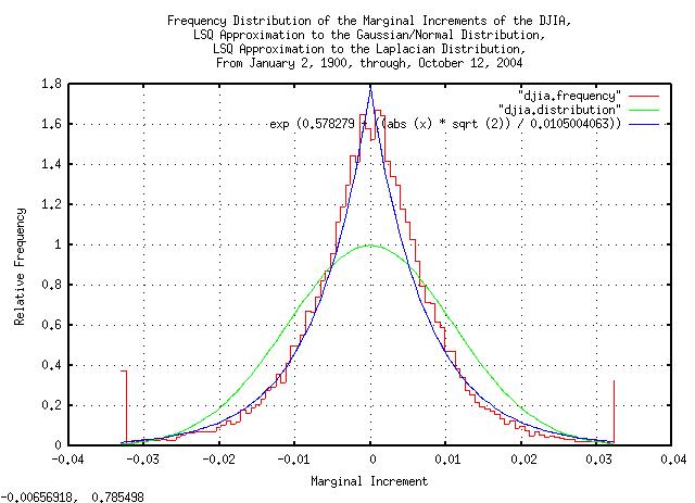
    egrep '^-' djia.frequency | tslsq -e -p | sed 's/ = .*$//'
    e^(0.578279 + 134.681795t)

    tsfraction djia | tsrms -p
    0.010998

And solving for the deviation, dev:



    sqrt (2) / dev = 134.681795
    dev = 0.0105004063

which is reasonably close to the root-mean-square calculated value, 0.010998.

And plotting:

Figure XVI

Figure XVI is a plot of the frequency distributions of the marginal increments of the DJIA's daily closes, from January 2, 1900, through, October 12, 2004, overlayed with the least-squares-best-fit Gaussian/Normal and Laplacian probability distributions.

For the Brownian motion/random walk fractal equivalent of the DJIA time series, as described in Section II, the marginal increments would simply be integrated, (or summed,) to obtain the deviation of the DJIA's value at some future time. Since the variance of the sum of random variables is the sum of the variances, and by the Central limit theorem, we would expect the deviations to add root-mean-square, and be Normally Distributed.

And verifying:



    tsmath -l djia | tslsq -o | tsrunmagnitude > djia.magnitude
    cut -f1 djia.magnitude | tsmath -l > temp.1
    cut -f2 djia.magnitude | tsmath -l > temp.2
    paste temp.1 temp.2 | egrep '^0-6\.' | tslsq -p
    -4.480455 + 0.515436t

And plotting:

Figure XVII

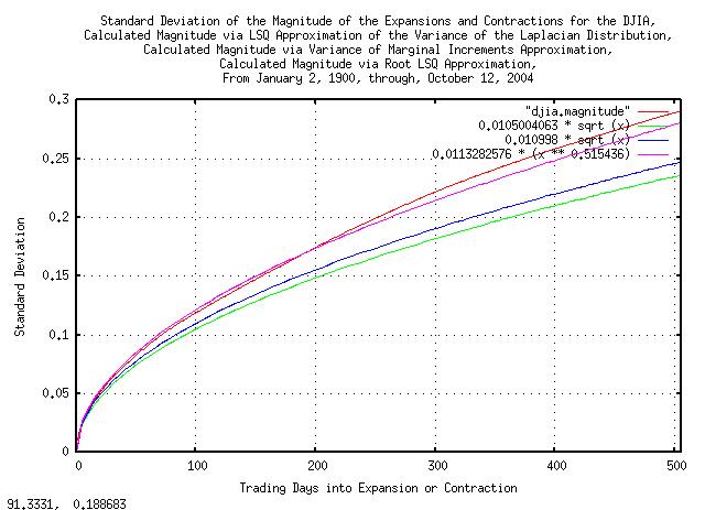
Figure XVII presents the standard deviation of the magnitude of the expansions and contractions of the Brownian motion/random walk equivalent of the time series for the DJIA, from January 2, 1900, through, October 12, 2004, the values as calculated from the least-squares-best-fit variance of the Laplacian Distribution, (0.0105004063 * sqrt (t),) the root-mean-square calculated value, (0.010998 * sqrt (x),) and the least-squares-best-fit function, (e^-4.480455 * (t^0.515436) = 0.0113282576 * (t^0.515436).

Appendix VI, Useful Approximations

For usual daily financial time series of non-linear high entropy economic systems with prediction times running less than about 20 days, (about a calendar month,) into the future using root-mean-square regression mathematics, the predicted risk is slightly larger than it really is, (by about 10%, or so, and leptokurtosis issues can usually be discounted as a mathematical expediency,) but for more than about 20 to days, (or, perhaps several hundred days in some circumstances,) the predicted risk is smaller, and leptokurtosis issues can not be ignored.

For prediction times running a calendar year, or more, into the future, leptokurtosis issues must be adequately addressed.


--

John Conover, john@email.johncon.com, http://www.johncon.com/

Last modified: Mon Jan 8 18:17:29 PST 2001 $Id: 041015122749.31772.html,v 1.0 2013/08/19 13:39:05 conover Exp $