|
From: John Conover <john@email.johncon.com>
Subject: Are the US Equity Markets Under Valued?
Date: 19 Aug 2002 08:39:21 -0000
Determination of the value of equity markets is difficult. But we
can gain some insight into the issues using the techniques offered in
the sections Quantitative
Analysis of Non-Linear High Entropy Economic Systems II and Quantitative
Analysis of Non-Linear High Entropy Economic Systems III, from the
Mathematical
Analysis & Numerical Methods series at the NdustriX
site. In the following analysis, the historical time series of the
DJIA, NASDAQ, and S&P500 indices through July 26, 2002 was
obtained from Yahoo!'s database of
equity Historical Prices,
(ticker symbols ^DJI, ^IXIC, and, ^SPC,
respectively,) in csv format-which was converted to a Unix
database format using the csv2tsinvest
program. (The converted DJIA time series,
djia1900-2002, started on
January 2, 1900, the NASDAQ,
nasdaq1984-2002, on October 11,
1984, and January 3, 1928 for the S&P500, file name,
sp1928-2002.)
The strategy of the analysis will be to convert the indices' time series into their Brownian motion/random walk fractal equivalents, and work with the Brownian motion statistics-since normal/Gaussian frequency distributions, (which are characteristic of Brownian motion,) are much more expedient to work with than the indices' characteristic log-normal frequency distributions. A short analysis of the limited precision available, (do to data set sizes,) of the statistics will be offered, followed by a Kalman filtering technique that will provide a methodology for the best possible accuracy for the current value of the markets, and statistics on how good the best possible accuracy is, which will be demonstrated in the conclusion.
Using standard statistical estimation techniques, (with a confidence level of at least one standard deviation, and an accuracy to within one standard deviation):
    tsfraction djia1900-2002 | tsstatest -c 0.841344746068542954 -e 0.00003680801891209803
    For a mean of 0.000232, with a confidence level of 0.841345
        that the error did not exceed 0.000037, 177081 samples would be required.
        (With 28047 samples, the estimated error is 0.000092 = 39.899222 percent.)
    For a standard deviation of 0.010988, with a confidence level of 0.841345
        that the error did not exceed 0.000037, 88541 samples would be required.
        (With 28047 samples, the estimated error is 0.000065 = 0.595169 percent.)

    tsfraction sp1928-2002 | tsstatest -c 0.841344746068542954 -e 0.00004125036602217883
    For a mean of 0.000260, with a confidence level of 0.841345
        that the error did not exceed 0.000041, 149462 samples would be required.
        (With 19802 samples, the estimated error is 0.000113 = 43.652147 percent.)
    For a standard deviation of 0.011313, with a confidence level of 0.841345
        that the error did not exceed 0.000041, 74731 samples would be required.
        (With 19802 samples, the estimated error is 0.000080 = 0.708319 percent.)

    tsfraction nasdaq1984-2002 | tsstatest -c 0.841344746068542954 -e 0.00007393334833205898
    For a mean of 0.000466, with a confidence level of 0.841345
        that the error did not exceed 0.000074, 73223 samples would be required.
        (With 4489 samples, the estimated error is 0.000299 = 64.043947 percent.)
    For a standard deviation of 0.014193, with a confidence level of 0.841345
        that the error did not exceed 0.000074, 36612 samples would be required.
        (With 4489 samples, the estimated error is 0.000211 = 1.487677 percent.)
Where the expected accuracy of the average,
avg, and deviation,
rms, of the marginal increments of the
indices' value, (for example, the DJIA's marginal increments are,
avg = 0.000232 and rms =
0.010988,) are shown. These two values are metrics
that determine the daily increase in value of the indices, (from the
Important
Formulas section of Quantitative
Analysis of Non-Linear High Entropy Economic Systems I,) and,
obviously, there is a problem with using the gain in an indices' value
as a metric-for example, although the DJIA has 28048 samples
represented, (over a century of daily closes,) the accuracy of the
measurement of avg is only within 40% of
the measured value for one standard deviation of the time!
Bottom line, any methodology that depends on measuring the increase
in gain of the marginal increments, (and thus
avg,) in an indices' value will lead to
inconsistent results-we can not find the median value of the indices
using any method that depends on avg
using the limited data sets at hand, (and this goes for intuition and
interpretation of graphs, too.) However, that the deviation of the
marginal increments, rms, converges to
respectable accuracies, quite quickly-which is exploitable.
Using the methodology described in Quantitative
Analysis of Non-Linear High Entropy Economic Systems III, and, Equation
(3.1), where it is shown that the accuracy of the metrics of the
median value, (which is the fair market value at the end of the time
series,) of the Brownian motion/random walk fractal equivalent of an
index will converge with a normal/Gaussian frequency distribution of
the error in the median value, (the convergence-the deviation of the
frequency distribution of the error-is, actually, rms *
erf (1 / sqrt (n)), for a data set size of
n, which is about rms * (1
/ sqrt (n)) for n >>
1, so we are working with the
rms, instead of
avg). Larger data sets will have a
smaller deviation around the mean, (which is the fair market value at
the end of the data set,) and smaller data sets will have a larger
deviation. It is the median value, and the distribution of its
measurement error, measured for all possible data set sizes that we
want to work with.
The following Unix Shell script, although not efficient, will suffice:
    #!/bin/sh
    #
    rm -f djia.jan.02.1900-jul.26.2002.histogram \
          sp.jan.03.1928-jul.26.2002.histogram \
          nasdaq.oct.11.1984-jul.26.2002.histogram
    #
    i=28048
    #
    while [ ${i} -gt 1 ]
    do
        tail -$i djia1900-2002 | tsmath -l | tslsq -o | \
            tail -1 >> djia.jan.02.1900-jul.26.2002.histogram
        i=`expr $i - 1`
    done
    #
    i=19308
    #
    while [ ${i} -gt 1 ]
    do
        tail -$i sp1928-2002 | tsmath -l | tslsq -o | \
            tail -1 >> sp.jan.03.1928-jul.26.2002.histogram
        i=`expr $i - 1`
    done
    #
    i=4490
    #
    while [ ${i} -gt 1 ]
    do
        tail -$i nasdaq1984-2002 | tsmath -l | tslsq -o | \
            tail -1 >> nasdaq.oct.11.1984-jul.26.2002.histogram
        i=`expr $i - 1`
    done
Where the tsmath
-l | tslsq
-o construct converts the log-normal characteristics
of the indices to their Brownian motion/random walk fractal
equivalents-there were 28048 trading days represented in the DJIA time
series, 19308 in the S&P, and, 4490 in the NASDAQ, and the script
walks through each time series, calculating the least squares
fit to the median, (fair market value,) for
n, n - 1,
n - 2
... 1 elements in the time series,
saving the final value of the median, (fair market value,) for each
iteration.
|
|
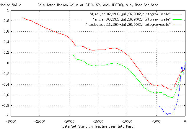
Figure I is a plot of the measured median, (i.e., fair market,)
value for the DJIA, S&P, and NASDAQ, as a function of data set
size, (the X-Axis was rescaled by subtracting the number of elements
in the time series from each X-Axis value for intuitive presentation,
aligning all graphs on the right, with time extending into the past to
the left.) For example, using a data set for the DJIA that ran from
15,000 days in the past, (January 20, 1944,) to the present, the
median value on July 26, 2002 would be measured as
e^0.279987 = 1.32311261176, or, the DJIA
would be calculated as being over valued by about 32%. Likewise, using
a data set that ran from 5,000 days in the past, (October 1, 1982,) to
July 26, 2002, the DJIA's median value would be measured as
e^-0.415470 = 0.660029994, or under
valued by about 34%. (The reason for the values around 0.8 for the
DJIA near time -30,000, is the Great Depression, where the DJIA lost
about 90% of its value, about a once-in-a millennia event, biasing the
data to smaller growth values for the entire century.)
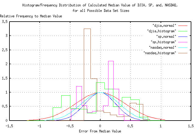
We now want to look at the frequency distribution of the measured median values in Figure I:
    tsnormal -s 17 -t djia.jan.02.1900-jul.26.2002.histogram > djia.normal
    tsnormal -s 17 -t -f djia.jan.02.1900-jul.26.2002.histogram > djia.histogram

    tsnormal -s 17 -t sp.jan.03.1928-jul.26.2002.histogram > sp.normal
    tsnormal -s 17 -t -f sp.jan.03.1928-jul.26.2002.histogram > sp.histogram

    tsnormal -s 17 -t nasdaq.oct.11.1984-jul.26.2002.histogram > nasdaq.normal
    tsnormal -s 17 -t nasdaq.oct.11.1984-jul.26.2002.histogram > nasdaq.histogram
And, plotting:
|
Figure II is a plot of the frequency distribution of the measured median, (i.e., fair market,) values in Figure I, for the DJIA, S&P, and NASDAQ, as a function of data set size-centered on the indices' measured median value on July 26, 2002 for comparison. Calculating the average, (i.e., mean = median,) and deviation:
    tsavg -p djia.jan.02.1900-jul.26.2002.histogram
    0.199951
    tsrms -p djia.jan.02.1900-jul.26.2002.histogram
    0.451294

    tsavg -p sp.jan.03.1928-jul.26.2002.histogram
    -0.225497
    tsrms -p sp.jan.03.1928-jul.26.2002.histogram
    0.335909

    tsavg -p nasdaq.oct.11.1984-jul.26.2002.histogram
    -0.712235
    tsrms -p nasdaq.oct.11.1984-jul.26.2002.histogram
    0.775733
(The median of the DJIA is 0.259990, -0.111612 for the S&P, and -0.858068 for the NASDAQ.)
On July 26, 2002, (converting the Brownian motion/random walk fractal equivalents back to their log-normal characteristics by exponentiating):
The DJIA's median value, (i.e., market value,) was
e^0.199951 = 1.22134291089, or about
22% over valued, and the high side deviation was
e^0.199951 + 0.451294 = 1.9236895833
and the low side, e^0.199951 - 0.451294 =
0.777789855, or the chances are one standard
deviation, (about 16%,) that the DJIA was over valued by more than
92%, or under valued by more than 12%.
The S&P's median value was e^-0.225497 =
0.798119455, or about 20% under valued, with a
high side deviation of e^-0.225497 + 0.335909 =
1.11673807178 and the low side,
e^-0.225497 - 0.335909 =
    0.570406508
, or the chances are one standard
deviation, or about 16%, that the S&P was over valued by at
least 12%, or under valued by at least 43%.
The NASDAQ's median value was e^-0.712235 =
0.4905466, or about 51% under valued, with a high
side deviation of e^-0.712235 + 0.775733 =
0.063498 and the low side,
e^-0.712235 - 0.775733 =
    0.225831078
, or the chances are one standard
deviation, or about 16%, that the NASDAQ was over valued by at
least 6%, or under valued by at least 77%.
So, as for the best assessment that can be made on whether the US equity markets were under valued on July 26, 2002, the answer is that they were probably close to fair market value, with both the DJIA and S&P within about 20% of being fair, meaning their median value, (the DJIA being slightly over valued, the S&P slightly under valued, by about 20%,) with the NASDAQ somewhat lower valued than the S&P at about 50% of fair value, (with the qualification that the limited data set size of the NASDAQ means that the number was more like numerology than science.)
The DJIA bottomed, during the Great Depression, on July 8, 1932. As it turns out, using this date as the start date in the time series for determining the fair market value of the DJIA and S&P works fairly well as representative of the conclusions, above:
    tail -18453 djia1900-2002 | tsmath -l | tslsq -o | tsmath -e > djia.jul.08.1932-jul.26.2002
    tail -18464 sp1928-2002 | tsmath -l | tslsq -o | tsmath -e > sp.jul.08.1932-jul.26.2002
and plotting:
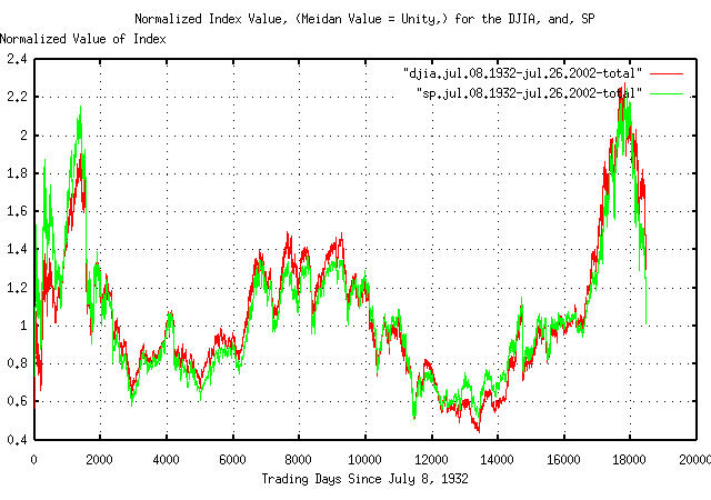
|
Figure III is a plot of the normalized value, (meaning the exponential curvature has been removed-or detrended,) for the DJIA and S&P indices, from July 8, 1932, to July 26, 2002. Values greater than unity mean the market is expanding faster than its median value, (i.e., in a bubble,) and is over valued, and less than unity, under valued. For example, around trading day 8,000 past July 8, 1932, (around January 11, 1961,) the DJIA and S&P were running about 20% over valued. Of interest is the bubble from around trading day 16,500, (about October 19, 1994.) This is the so-called dot-com bubble. Note that it was not necessarily unique in the last 70 years-the bubble coming out of the Great Depression, (on trading days 0-2,000, or about July 8, 1932 to March 27, 1939,) was almost as significant, (both had magnitudes, where the market was over valued by a factor of slightly more than two,) and the market value of the run up prior to the Crash of 1929 was over valued by almost a factor of two, also.
So, the claim that the dot-com era was the greatest wealth generator in the last century is a myth. It was only one of a few, (but was not the greatest-the period between trading day 6,500 and 10,000 holds that honor, about January 27, 1955 to January 29, 1969; the market was only about 20% over valued, but the bubble lasted fourteen years. Typical bubbles last only about four years-as did the dot-com bubble.) Of passing interest is the negative bubbles from trading day 2,000 through 6,500 and 11,000 through 15,000, (March 27, 1939 through January 27, 1955 and January 17, 1973 through November 14, 1988,) where the markets were about 40% under valued. (The period from trading day 14,500 through 16,000 is interesting, too-the market was at its fair market median for almost six years, November 21, 1986 though October 28, 1992.)
At any rate, the intuitionist can conjure up a rationale for all the bubbles of the last seventy years, based on the prevailing dogma, (i.e., depending on who is telling the story.)
Which leads me to a closing remark about such things. Suppose that one was to assume that the data set from October 11, 1984 to July 26, 2002, (just under 18 calendar years,) was adaquate to determine what the US markets were doing:
    #!/bin/sh
    #
    tail -18453 djia1900-2002 | tsmath -l | tslsq -o | tail -4490 | tsmath -e > djia.jul.08.1932-jul.26.2002
    tail -18464 sp1928-2002 | tsmath -l | tslsq -o | tail -4490 | tsmath -e > sp.jul.08.1932-jul.26.2002
    #
    tail -4490 djia1900-2002 | tsmath -l | tslsq -o | tsmath -e > djia.oct.11.1984-jul.26.2002
    tail -4490 sp1928-2002 | tsmath -l | tslsq -o | tsmath -e > sp.oct.11.1984-jul.26.2002
    tail -4490 nasdaq1984-2002 | tsmath -l | tslsq -o | tsmath -e > nasdaq.oct.11.1984-jul.26.2002
And plotting:
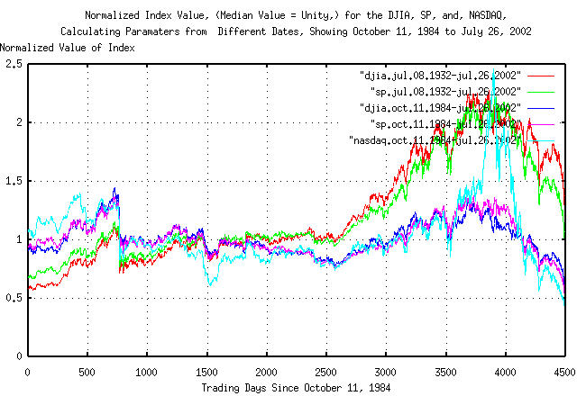
|
Figure IV is the last 4490 trading days, (i.e., trading days between October 11, 1984 and July 26, 2002,) of Figure III, and for comparison, imposed on graphs made by using the exact same methodology, but using only data sets for the DJIA, S&P, and NASDAQ, of the 4490 trading days, since October 11, 1984. Note how easy it is to jump to the conclusion that the markets are in terrible shape, and under valued by almost 50%.
Its always easy to find statistical significance where there isn't any.
--

John Conover, john@email.johncon.com, http://www.johncon.com/