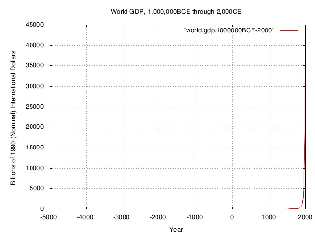
World Gross Domestic Product

The GDP metric is in 1990 Nominal International Dollars, and is in real dollars, relative to the value of the US dollar in 1990.

Figure I is a plot of the World GDP, 1,000,000BCE through 2,000CE, in 1990 International Dollars. The World GDP is shown only since the late stone age, about -5,000BCE. Note the hockey stick of the exponential increase of the World GDP.

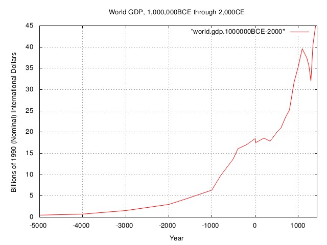
Figure II is the same plot of the World GDP, 1,000,000BCE through 2,000CE, in 1990 International Dollars. The World GDP is shown only since the late stone age, about -5,000BCE, with the ordinate expanded for clarity.

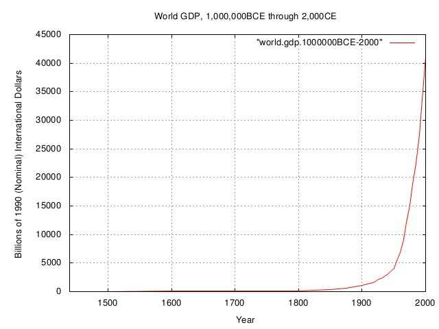
Figure III is the same plot of the World GDP, 1,000,000BCE through 2,000CE, in 1990 International Dollars. The World GDP shown includes only the modern economy, about the Sixteenth Century CE.

World Population

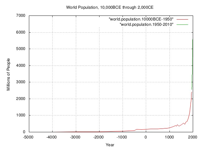
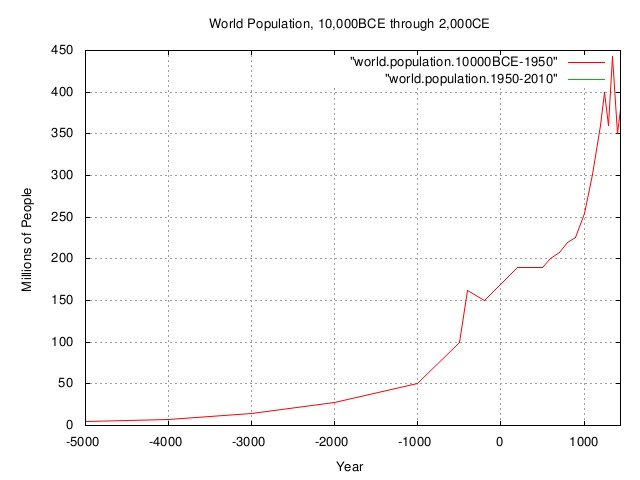
Figure IV is a plot of the World Population, 10,000BCE through 2,010CE. The World Population is showen only since the late stone age, about -5,000BCE. Note the concatenation of UN data past 1950.

Figure V is the same plot of the World Population, 10,000BCE through 2,010CE. The World Population shown is only up to the the modern economy, about the Sixteenth Century CE.

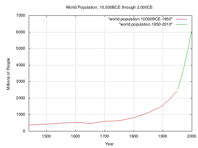
Figure VI is the same plot of the World Population, 10,000BCE through 2,010CE. The World Population shown includes only the modern economy, from about the Sixteenth Century CE.

World Gross Domestic Product per Capita

Note that this is an analysis of the World GDP per capita, (using the mean GDP per capita, as opposed to the median GDP per capita, which, alas, is not available, and is the World GDP divided by the World Population.)

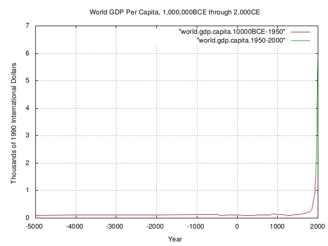
Figure VII is a plot produced by dividing the World GDP by the World Population, and is the mean GDP per capita, 10,000BCE through 2,000CE. Clearly, the standard of living didn't change from subsistence levels, (the so called Malthusian stagnation, proposed by Thomas Robert Malthus, 1766-1834,) until the advent of the modern economy, about the Sixteenth Century CE.

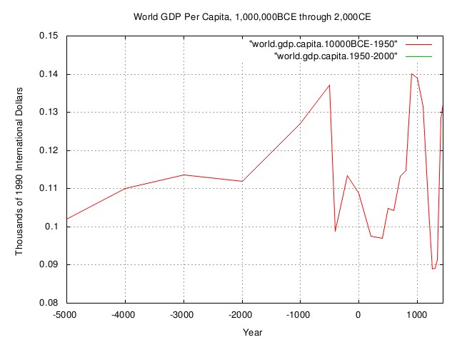
Figure VIII is the same plot produced by dividing the World GDP by the World Population, and is the mean GDP per capita, 10,000BCE through 2,000CE, but values past the Sixteenth Century, the beginning of the modern economy, have been truncated. Clearly, the standard of living didn't change from subsistence levels until the advent of the modern economy.

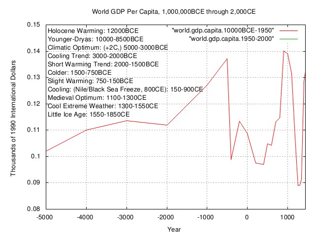
Figure IX is the same plot produced by dividing the World GDP by the World Population, and is the mean GDP per capita, 10,000BCE through 2,000CE, but values past the Sixteenth Century, the beginning of the modern economy, have been truncated. Clearly, the standard of living didn't change from subsistence levels until the advent of the modern economy. Temperature observations from holocene.climate.txt were added, and will be persued further on in the study.

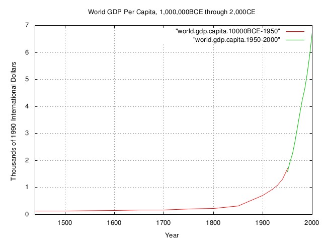
Figure X is the same plot produced by dividing the World GDP by the World Population, and is the mean GDP per capita, 10,000BCE through 2,000CE, but only values past the Sixteenth Century, the beginning of the modern economy, are shown. Clearly, the standard of living started to increase, rapidly, from many millennia of stagnation at subsistence levels, with the advent of the modern economy.

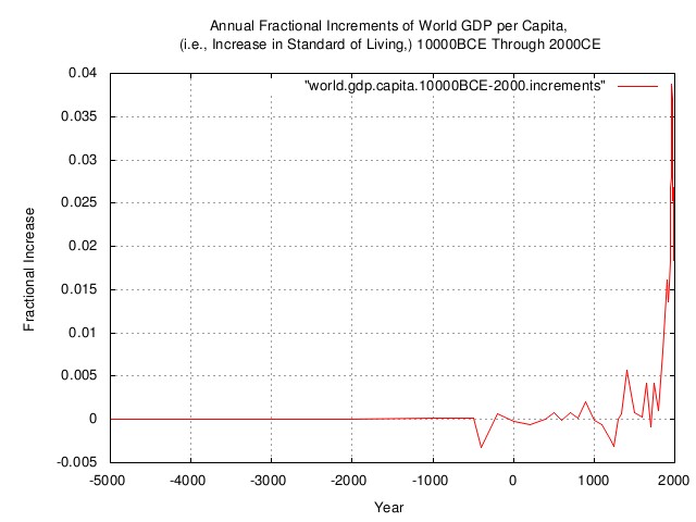
Figure XI is the annual fractional increments of the world GDP per capita, (i.e., dividing the World GDP by the World Population, and is the mean GDP per capita, 10,000BCE through 2,000CE, annualized, to provide the increase in the standard of living per year.) The beginning of the modern economy, is clearly evident.

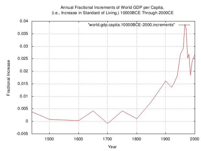
Figure XII is the annual fractional increments of the world GDP per capita, (i.e., dividing the World GDP by the World Population, and is the mean GDP per capita, 10,000BCE through 2,000CE, annualized, to provide the increase in the standard of living per year,) but only values past the Sixteenth Century, the beginning of the modern economy, are shown.

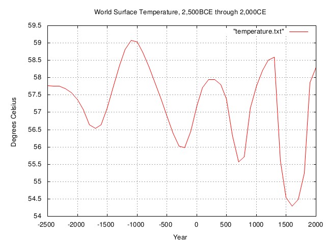
Figure XIII is a plot of the World's surface temperature, 2,500BCE through 2,000CE.

    tsmath -t -l temperature.txt | tsderivative -t | tsavg -p
    0.000202
    tsmath -t -l temperature.txt | tsderivative -t | tsrms -p
    0.013498
              

    avg=0.000202
    rms=0.013498
    P(avg,rms)
            0.50748259001333530893 .................................(B-1.24)

              

    tsfraction -t temperature.txt | tsavg -p
    0.000293
    tsfraction -t temperature.txt | tsrms -p
    0.013471

              

    avg=0.000293
    rms=0.013471
    P(avg,rms)
            0.51087521342142379927 .................................(B-1.24)

              

    (2 * P ) - 1 = 2 * 0.51 - 1 = 0.02 .............................(B-1.18)

              

    G = (1 + rms)^P * (1 - rms)^(1 - P) = 1.00020229603023145739 ...(B-1.20)

              

    tslsq -e -p temperature.txt
    e^(4.044849 + -0.000006t)

              

    exp(4.044849)
            57.10256289611706131889

    exp(-0.000006)
            0.999994000017999964

              

Note that photo synthesis is a chemical process. The Arrhenius Equation determines the reaction rate of a chemical process as a function of temperature, so agricultural production should be coherent with temperature. (Of course, the climate is a complex system, and depends on many variables-however, temperature is among the most significant.)

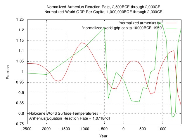
Figure XIV is a plot of the Arrhenius reaction rate, and, the mean World GDP per capita, both LSQ normalized to unity over the interval of 2,500BCE to 2,000CE.

It appears that there is a correlation, but the temperature data seems to be shifted a couple of centuries, (which is not uncommon due to data processing/smoothing at the millennia level.) In a private correspondence with Randy Mann, (Long Range Weather), it is possible the shift is a data processing artifact.

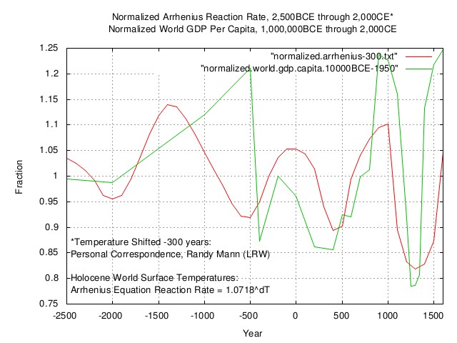
Figure XV is a plot of the Arrhenius reaction rate, and, the mean World GDP per capita, both LSQ normalized to unity over the interval of 2,500BCE to 2,000CE, with the temperature shifted 3 centuries.

It does appear that throughout the history of civilization, GDP was dominated by agricultural production, (at least until the advent of the modern economy,) placing humanity at the whim of the weather.

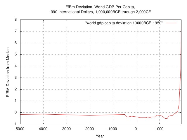
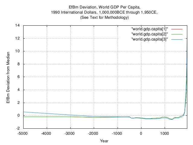
Figure XVI is a plot of the deviation from the median of the arithmetic fractional Brownian motion equivalent of mean World GDP per capita, from the stone age, about -5000BCE, through 2000CE. (For details, see: Quantitative Analysis of Non-Linear High Entropy Economic Systems II.) This methodology is useful for studying bubbles in geometric Brownian motion fractal time series.

Figure XVII is a plot of the deviation from the median of the arithmetic fractional Brownian motion equivalent of mean World GDP per capita, from the stone age, about -5000BCE, through 2000CE. (For details, see: Quantitative Analysis of Non-Linear High Entropy Economic Systems II.) There are several techniques for deriving the arithmetic fractional Brownian motion equivalent from the geometric fractal, and all produce equivalent results, within reason, (if the time series really is a geometric fractional Brownian motion process.) Most of the techniques involve taking the logarithm of the time series, (as opposed to working with the marginal increments.)

The World GDP data is not a pure time series, (the early data is spotty,) but this verifies that techniques involving the logarithm are, at least reasonably so, valid.

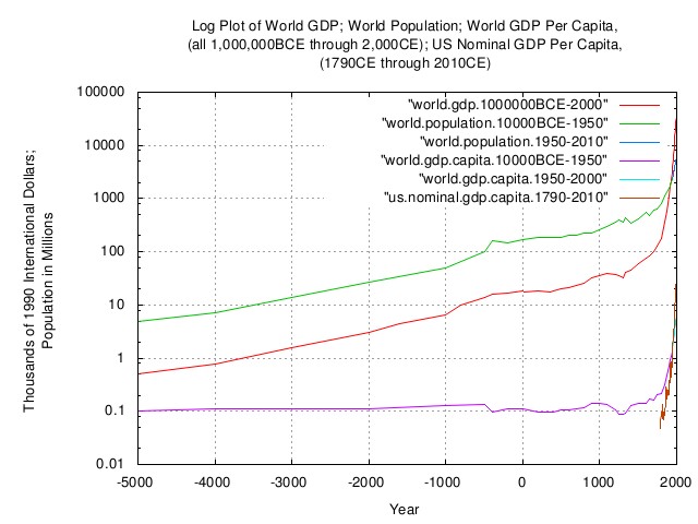
Figure XVIII is a log-log plot of the mean World GDP per capita, -5,000BCE, the late stone age, through 2,000CE. Included variables are the World GDP, the World population, and the US nominal GDP since 1790, (converted to 1990 International Dollars.)

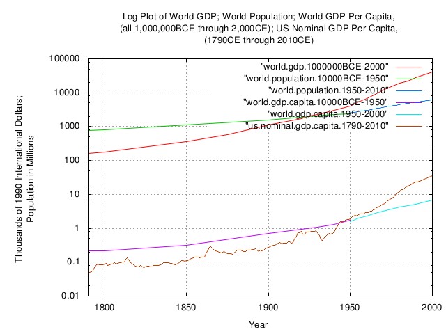
Figure XVIV is the same log-log plot of the mean World GDP per capita, -5,000BCE, the late stone age, through 2,000CE, but showing only the late 1700s through 2,000CE. Included variables are the World GDP, the World population, and the US nominal GDP since 1790, (converted to 1990 International Dollars.) Notice the concatenation of data for the World population with UN data past 1950.

Of interest is the comparison of the mean GDP per capita of the US and the mean GDP per capita of the world, prior to about 1950, i.e., post WWII. Of further interest is the inflection in the US GDP per capita about 1974.

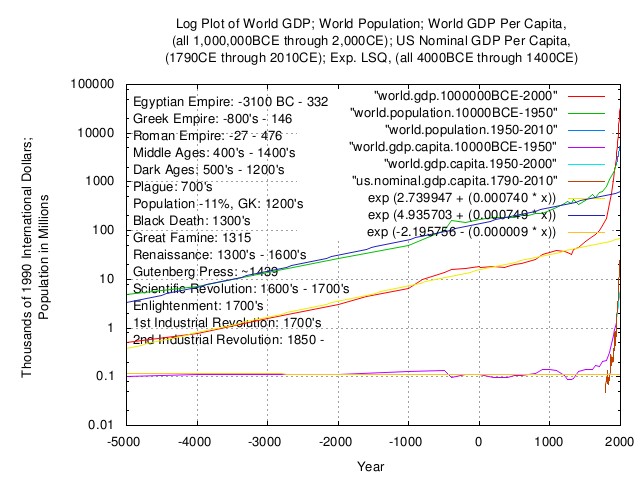
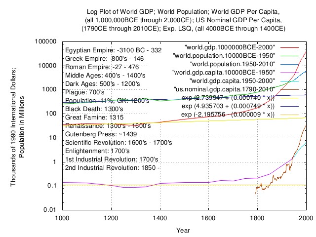
Figure XX is the same log-log plot of the mean World GDP per capita, -5,000BCE, the late stone age, through 2,000CE. Included variables are the World GDP, the World population, and the US nominal GDP since 1790, (converted to 1990 International Dollars.) Additionally, historical comments of the era are added, for convenience, and, LSQ approximations to the curves.

Figure XXI is the same log-log plot of the mean World GDP per capita, -5,000BCE, the late stone age, through 2,000CE. The plot is centered around the start of the modern economy. Included variables are the World GDP, the World population, and the US nominal GDP since 1790, (converted to 1990 International Dollars.) Additionally, historical comments of the era are added, for convenience, and, LSQ approximations to the curves.

It would appear that from, at least, -5,000BCE, the late stone age, to the early 1600s CE, the mean World GDP per capita remained constant, at about subsistence levels. In the early 1600s, (depending on who's calibrated eye is telling the story,) the modern economy began, and the GDP per capita, i.e., the standard of living, started increasing at an exponential rate. This would be coincident with the Scientific Revolution.

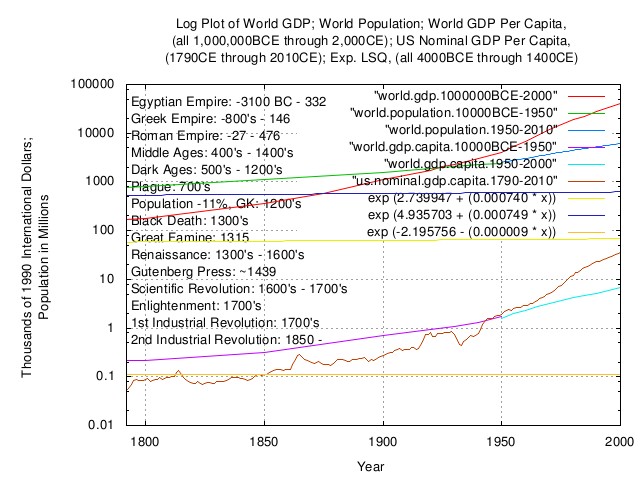
Figure XXII is the same log-log plot of the mean World GDP per capita, -5,000BCE, the late stone age, through 2,000CE. The plot is centered later, around the late 1800s, well into the advent of the modern economy. Included variables are the World GDP, the World population, and the US nominal GDP since 1790, (converted to 1990 International Dollars.) Additionally, historical comments of the era are added, for convenience, and, LSQ approximations to the curves.

Up to this point in the study of the mean World GDP per capita, the assumption is that the GDP system was a geometric fractional Brownian motion process, which is often used, (at least as an approximation,) for analyzing the data from complex systems. Numerically, there are but small differences between a geometric fractional Brownian motion process, and a non-linear dynamical system, (usually a relatively small negative parameter in the marginal increments of the data.) Proceeding on that assumption, the simplest chaotic system is the Logistic Function, (also called the discreet time parabolic function in Europe,) which has a single Strange Attractor. In addition to initially exhibiting exponential characteristics, the Logistic Function is S shaped, over time.

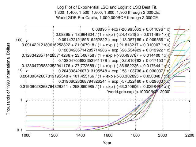
Figure XXIII is a log-log plot of the mean World GDP per capita, -5,000BCE through 2,000CE, and several exponential and logistic LSQ approximations to the data, centered around the advent of the modern economy. The LSQ approximations were iterated at approximately century intervals for best fit candidates, and extrapolated to 2,200CE.

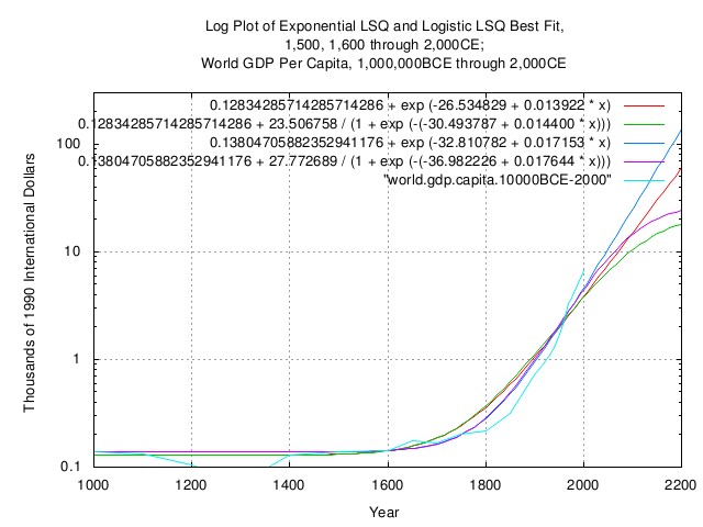
Figure XXIV is the same log-log plot of the mean World GDP per capita, -5,000BCE through 2,000CE, and two best exponential LSQ approximation candidates, and, the two best logistic LSQ approximation candidates, centered around the advent of the modern economy. The LSQ approximations were extrapolated to 2,200CE.

The logistic function analysis will be pursued from here on.

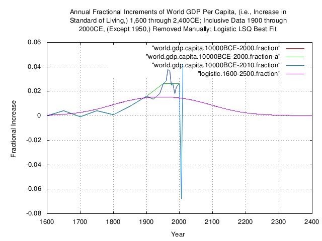
Figure XXV is a plot of the annual fractional increments, (i.e., marginal increments,) of the mean World GDP per capita, -5,000BCE through 2,000CE, and the fractional increments of the best logistic LSQ approximation candidate, centered around 2,000CE. The analysis was done on half century data, and extrapolated to 2,400CE.

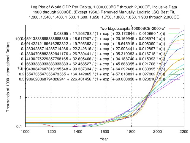
Figure XXVI is a log-log plot of the mean World GDP per capita, -5,000BCE through 2,000CE, and several logistic LSQ approximations to the data, centered around the advent of the modern economy. The LSQ approximations were iterated as shown for best fit candidates, and extrapolated to 2,200CE. The analysis was done on half century data.

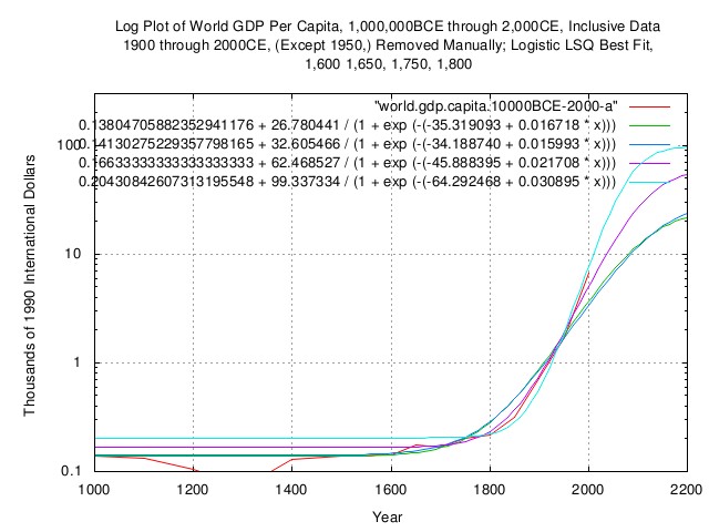
Figure XXVII is the same log-log plot of the mean World GDP per capita, -5,000BCE through 2,000CE, and the four best LSQ approximations to the data, centered around the advent of the modern economy, and extrapolated to 2,200CE.

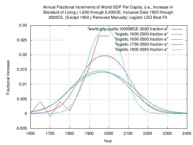
Figure XXVIII is a plot of the fractional increments, (i.e., marginal increments,) of the mean World GDP per capita, -5,000BCE through 2,000CE, and the fractional increments of the four best LSQ approximations to the data, centered around 2,000CE, and extrapolated to 2,400CE.

Note that this establishes a plausibility that the mean World GDP per capita is a non-linear dynamical system process, which is of little value. The probability that it is is more useful.

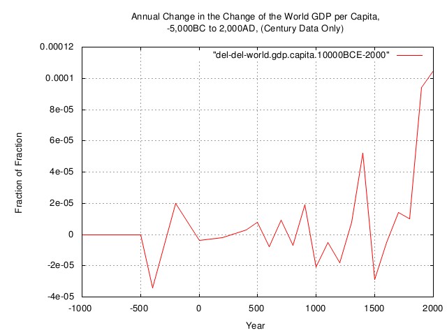
Figure XXIV is a plot of the change in the change of the mean World GDP per capita, -5,000BCE through 2,000CE, based on century data.

Archive

The data presented here can be reconstructed, in its entirety, from the historical.economics.tar.gz tape archive file, which contains all data and references, thereto. The source code to all programs used in the analysis is available from the NtropiX site, tsinvest.tar.gz, and, the NdustrixX site, fractal.tar.gz, tape archive files. All use the "standard" Unix development systems of rcs(1) and make(1) to facilitate replication.

It should be noted that many of the data set sizes are pitifully small-some as few as two hundred data points, (a standard error of about 7% of the standard deviation,) and conclusions can only be regarded as circumstantial.

License

The information contained herein is private and confidential and dissemination is strictly forbidden, except under the provisions of contractual license.

THE AUTHOR PROVIDES NO WARRANTIES WHATSOEVER, EXPRESSED OR IMPLIED, INCLUDING WARRANTIES OF MERCHANTABILITY, TITLE, OR FITNESS FOR ANY PARTICULAR PURPOSE. THE AUTHOR DOES NOT WARRANT THAT USE OF THIS INFORMATION DOES NOT INFRINGE THE INTELLECTUAL PROPERTY RIGHTS OF ANY THIRD PARTY IN ANY COUNTRY.

So there.

Copyright © 1992-2016, John Conover, All Rights Reserved.

Comments, questions, and problem reports should be addressed to:

john@email.johncon.com

http://www.johncon.com/john/

http://www.johncon.com/ntropix/

http://www.johncon.com/ndustrix/

http://www.johncon.com/nformatix/

http://www.johncon.com/ndex/