|
From: John Conover <john@email.johncon.com>
Subject: Quantitative Analysis of Non-Linear High Entropy Economic Systems VII
Date: 28 Aug 2006 09:39:47 -0000
As mentioned in Section I, Section II, Section III, Section IV, Section V and Section VI, much of applied economics has to address non-linear high entropy systems-those systems characterized by random fluctuations over time-such as net wealth, equity prices, gross domestic product, industrial markets, etc.
A quick review of this series.
Many economic systems are characterized by non-linear high entropy time series. These time series are a geometric progression, as analyzed in Section I, and the distribution of the marginal increments of the time series exhibit log-normal distributions, as suggested in Section II. The characteristics of the marginal increments can be analyzed as suggested in Section III, and, Section IV, to formulate investment strategies and optimizations as illustrated in Section V. The finer details of the types of leptokurtosis found in the marginal increments of financial time series is analyzed in Section VI.
Revisiting the DJIA, (since it has a long historical database,) a meticulous analytical approach will be used to analyze the characteristics of the closing values of the DJIA. The analytical procedure will use a conscientious process commonly used in engineering practice:
script
of analytical
programs, "chained" together, (usually with Unix
pipes for maintainability and extensibility.)Note: the C source code to all programs used in the
script
are available from the NtropiX Utilities
page, or, the NdustriX Utilities
page, and is distributed under License.
The historical time series of the DJIA index was obtained from Yahoo!'s database of equity Historical Prices, (ticker
symbols ^DJI,) in csv format. The csv
format was converted to a Unix database,
djia, using the csv2tsinvest
program. (The DJIA time series started on January 2, 1900, and
contained 29010 daily closes, through May 26, 2006.)
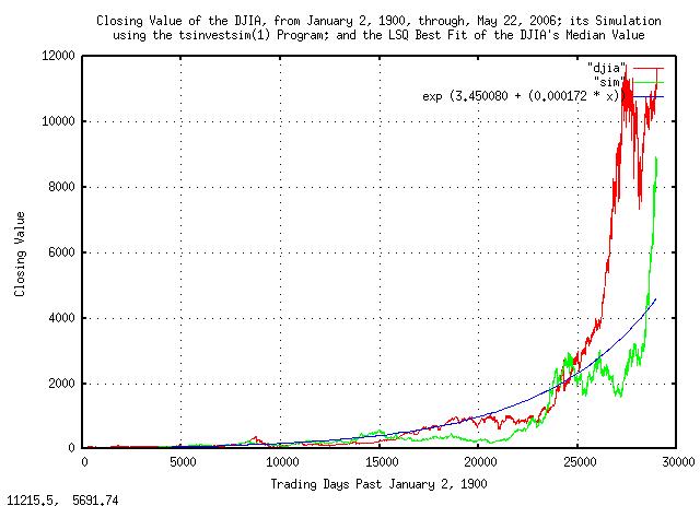
Plotting the closing values of the DJIA:
|
|
Figure I is a plot of the daily closes of the DJIA, from January 2,
1900, through, May 26, 2006. The simulated value is constructed from
the variables extracted from the empirical data in the
script,
below, as is the median value, and presented here for comparison.
The script
used for the programs will be walked through statement by
statement, to illustrate and validate the analytic procedure.
Starting with the first two statements, and following the outline from Section I:
    tsfraction djia | tsavg -p
    0.000236
    tsfraction djia | tsrms -p
    0.010950
From Equation
(1.24), P = 0.51077625570776255708,
meaning that there are, on average, about
51 up movements, and
49 down movements, out of one
hundred. P is the probability of an up
movement in the DJIA.
Log-normal distributions of the marginal increments of a time series-those distributions commonly found in geometric progressions-are difficult to comprehend intuitively, and it is expedient to convert the time series to its Brownian Motion, (random walk,) equivalent as outlined in Section II.
The root-mean-square, rms, of the
Brownian Motion equivalent, (the next two statements in the
script):
    tsfraction djia | tsmath -s 0.000236 | tsrms -p
    0.010947
    tsmath -l djia | tsderivative | tsmath -s 0.000176 | tsrms -p
    0.010998
which are alternative methods-the first extracts the
rms directly from the geometric
progression, and the second from its Brownian Motion equivalent. The
two answers should be nearly identical. The offset, avg
= 0.000236, is subtracted from the first, and
ln (g) = ln (1.000176) = 0.000176 from
the second. The logarithm of the rms
will be useful later, ln (0.010947) =
-4.51468983285971677053.
The number of elements in the time series, and its beginning value will be of interest, later:
wc djia
29010 29010 202761 djia
head -1 djia
68.13
The marginal gain, g of the Brownian
Motion equivalent is determined by the next two statements in the
script:
tsgain -p djia
1.000176
tsmath -l djia | tsderivative | tsavg -p
0.000176
tslsq -e -p djia
e^(3.450080 + 0.000172t) = 1.000172^(20062.070643 + t) = 2^(4.977413 + 0.000248t)
The two answers should be nearly equivalent. The third line in this
section of the script provides yet another method-it uses the
exponential Least-Squares, (LSQ,) best fit to the original time
series; it, too, should provide a nearly identical answer to the to
the other two methods, (0.000176
vs. 0.000172.) The LSQ best fit to the
data starts with a first element value of exp (3.450080)
= 31.50291244093657542517.
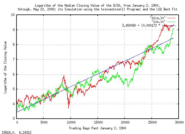
Using the variables produced by the LSQ best-fit, and plotting the Brownian Motion equivalent of the DJIA:
|
Figure II is a plot of the Brownian Motion, (random walk,)
equivalent of the DJIA, from January 2, 1900, through, May 26,
2006. The simulated values are constructed from the variables
extracted from the empirical data in the script,
below.
Having converted the DJIA's time series to its Brownian Motion equivalent, the marginal increments can be analyzed. One of issues to be addressed is leptokurtosis-specifically, the deviation from the theoretical assumption that the increments are statistically independent-this will indicate what math should be used, (if the increments are independent, then root-mean-square should be used, if not, another root-mean should be used, as per Section VI.) An iterated script will be used to find the root:
R="0.5"
#
> "log"
#
LAST="NOTHING"
#
LOOP="1"
#
while [ "${LOOP}" -eq "1" ]
do
tsmath -l djia | tsderivative | tsmath -s 0.000176 | tsintegrate | \
tsrunmagnitude -r "${R}" > "djia.magnitude"
cut -f1 "djia.magnitude" | tsmath -l > "temp.5"
cut -f2 "djia.magnitude" | tsmath -l > "temp.6"
LAST=`paste temp.5 temp.6 | egrep '^[0-5]\.' | tslsq -p`
echo "${LAST}"
R=`echo "${LAST}" | sed -e 's/^.* //' -e 's/t.*$//'`
#
if grep -e "${LAST}" "log"
then
LOOP="0"
fi
#
mv "temp.5" "temp.5.last"
mv "temp.6" "temp.6.last"
mv "djia.magnitude" "djia.magnitude.last"
echo "${LAST}" >> "log"
done
The script
fragment is an iterated search-for-solution algorithm that initially
assumes a root of 0.5, uses
tsrunmagnitude
to analyze the time series and produce a more accurate approximation
to the root, and so on, until no further improvements were
possible. (The other statements in the loop are standard Unix text
database manipulations, using
cut(1) and
paste(1) to extract, and
reassemble fields in the database,
egrep(1) to extact only days
1 - e^5.999... = 403 days, and so
forth.)
The output of the script
fragment is:
-4.592316 + 0.537435t
-4.648576 + 0.541035t
-4.653584 + 0.541347t
-4.654019 + 0.541375t
-4.654057 + 0.541377t
-4.654058 + 0.541377t
-4.654058 + 0.541377t
meaning that, at least in the very short term, (i.e., daily
returns,) there is about a 54% chance
that what happened on any one day will occur on the next day,
also.
The simulation can now be constructed using the tsinvestsim
program with the file,
djia.sim:
djia, p = 0.51077625570776255708, f = 0.010950, i = 31.50291244093657542517, h = 0.541377, l = 1
and running the tsinvestsim:
tsinvestsim djia.sim 29010 | cut -f3 > sim
And, analyzing the simulation file,
sim, in an identical manner to
the DJIA analysis:
tsfraction sim | tsavg -p
0.000253
tsfraction sim | tsrms -p
0.010994
tsmath -l sim > sim.ln
tslsq -e -p sim
e^(3.548001 + 0.000146t) = 1.000146^(24382.768809 + t) = 2^(5.118683 + 0.000210t)
Which compares favorably to the original analysis of the DJIA. The files produced in the simulation were presented in Figure I and Figure II, above, for comparison with the original DJIA time series.
The ground work is now prepared to look into issues of leptokurtosis of the DJIA. As presented in Section VI, the model used will be Laplacian distribution:
tsfraction djia | tsmath -s 0.000236 | tsnormal -t > djia.distribution
tsfraction djia | tsmath -s 0.000236 | tsnormal -t -f > djia.frequency
tsfraction sim | tsmath -s 0.000236 | tsnormal -t > sim.distribution
tsfraction sim | tsmath -s 0.000236 | tsnormal -t -f > sim.frequency
egrep '^-' djia.frequency | wc
50 100 950
egrep '^-' djia.frequency | tail -49 | tslsq -e -p | sed 's/ = .*$//'
e^(0.710298 + 147.146009t)
Here, the offset of distribution is subtracted, as above, from the
marginal increments of the DJIA's value, and its simulation, and a
histogram of the marginal increments made with the tsnormal
program. An LSQ approximation to the distribution is necessary, and
since the Laplace distribution is a double exponential, the negative
side of the distribution is omitted using
egrep(1), and the
tslsq
program used to provide the LSQ best-fit approximation to the
distribution. And plotting:
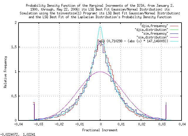
|
Figure III is a plot of the distribution of the marginal increments of the Brownian Motion, (random walk,) equivalent of the DJIA, from January 2, 1900, through, May 26, 2006, and its simulation. The Gaussian/Normal LSQ best-fit approximation is presented as a comparison, also-the variance of all distributions shown is nearly identical, as would be expected.
Integrating the count of marginal increments in each
0.1% "bucket" to obtain the
cumulative probabilities:
tsfraction djia | tsmath -s 0.000236 | sed 's/[0-9][0-9][0-9]$//' | sort -n | \
tscount -r | tsmath -t -d 29009 | tsintegrate -t > djia.cumulative
tsfraction sim | tsmath -s 0.000236 | sed 's/[0-9][0-9][0-9]$//' | sort -n | \
tscount -r | tsmath -t -d 29009 | tsintegrate -t > sim.cumulative
And plotting:
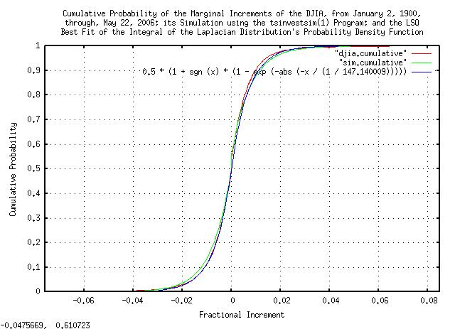
|
Figure IV is a plot of the cumulative distribution of the marginal increments of the Brownian Motion, (random walk,) equivalent of the DJIA, from January 2, 1900, through, May 26, 2006, and its simulation. It was analyzed by a different method-its derivative should be much the same as Figure III, above, and is included as a method of cross-checking the data and analysis.
The run lengths of the expansions and contractions of the DJIA:
tsmath -l djia | tsderivative | tsmath -s 0.000176 | tsintegrate | tsrunlength | cut -f1,7 > djia.length
tsmath -l sim | tsderivative | tsmath -s 0.000176 | tsintegrate | tsrunlength | cut -f1,7 > sim.length
And, plotting:
|
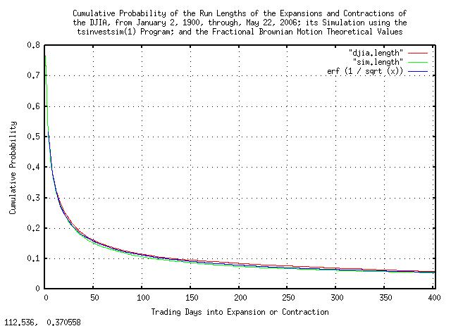
Figure V is a plot of the cumulative probability of the run lengths
of the expansions and contractions of the Brownian Motion, (random
walk,) equivalent of the DJIA, from January 2, 1900, through, May 26,
2006, and its simulation. erf (1 / sqrt
(x)) is the theoretical value. As an example
interpretation, there is a little over
10% chance of a the value of the DJIA
being above its median value for at least
100 trading days.
And, the magnitude of the expansions and contractions of the DJIA:
tsmath -l djia | tsderivative | tsmath -s 0.000176 | tsintegrate | tsrunmagnitude > djia.magnitude
tsmath -l sim | tsderivative | tsmath -s 0.000176 | tsintegrate | tsrunmagnitude > sim.magnitude
And, plotting:
|
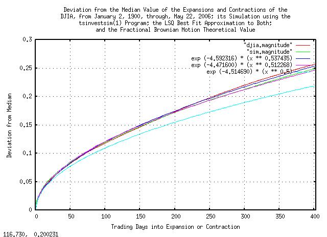
Figure VI is a plot of the deviation from the median value of the
expansions and contractions of the Brownian Motion, (random walk,)
equivalent of the DJIA, from January 2, 1900, through, May 26, 2006,
and its simulation. 0.010947 * sqrt (x)
is the theoretical value. As an example interpretation, there is a
standard deviation chance that the value of the DJIA will be within a
little more than +/- 10% of its median
value at 100 trading days.
The discrepancies of the curves from the theoretical values are do
to market inefficiencies. The empirical curves are steeper
for small time intervals, (near 1 day,) because the market does not
respond instantaneously to new information-there is a slight
persistence from one day to the next. Additionally, the
empirical curves are steeper than the theoretical at
253 trading days, (about a calendar
year,) for structural reasons-specifically, taxation
schedules that favor funds selling off losing equities before the end
of the calendar year. It should be noted that deviation from the
theoretical values is not constant, and varies throughout the calendar
year. The LSQ best fit approximations are an average over the
403 days-about
19 months.
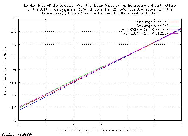
Market inefficiencies are exploitable, (if the DJIA were a perfect Brownian Motion random walk, the market would be fair, and no one could have an advantage over anyone else in the long run.) Delving into the market inefficiencies by making a log-log plot of Figure VI.
cut -f1 djia.magnitude | tsmath -l > temp.1
cut -f2 djia.magnitude | tsmath -l > temp.2
paste temp.1 temp.2 > djia.magnitude.ln
cut -f1 sim.magnitude | tsmath -l > temp.3
cut -f2 sim.magnitude | tsmath -l > temp.4
paste temp.3 temp.4 > sim.magnitude.ln
egrep '^[0-5]\.' djia.magnitude.ln | tslsq -p
-4.592316 + 0.537435t
egrep '^[0-5]\.' sim.magnitude.ln | tslsq -p
-4.471600 + 0.512268t
And, plotting:
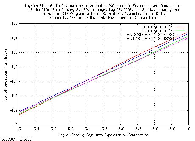
|
Figure VII is a log-log plot of the deviation from the median value of the expansions and contractions of the Brownian Motion, (random walk,) equivalent of the DJIA, from January 2, 1900, through, May 26, 2006, and its simulation shown in Figure VI.
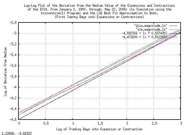
And, plotting Figure VII for short time intervals to emphasize the market inefficiency:
|
Figure VIII is a log-log plot of the deviation from the median value of the expansions and contractions of the Brownian Motion, (random walk,) equivalent of the DJIA, from January 2, 1900, through, May 26, 2006, and its simulation, plotted for a few trading days.
And, plotting Figure VII around a calendar year to emphasize the market inefficiency:
|
Figure IX is a log-log plot of the deviation from the median value of the expansions and contractions of the Brownian Motion, (random walk,) equivalent of the DJIA, from January 2, 1900, through, May 26, 2006, and its simulation, plotted at a calendar year.
Figure VIII and Figure IX indicate exploitable market inefficiencies-where the marginal increments are not statistically independent, (iid,) meaning some sense of predictability.
To remove the statistical dependence, the marginal increments of the Brownian Motion, (random walk,) equivalent of the DJIA can be moved randomly, (i.e., scrambled,) in the time series, and the random walk equivalent of the time series re-assembled, then the deviation from the median value of the expansions and contractions analyzed:
#
tsmath -l djia | tsderivative | tssequence | sort -n | cut -f3 | \
tsmath -s 0.000176 | tsintegrate > "scrambled"
#
R="0.5"
#
> "log"
#
LAST="NOTHING"
#
LOOP="1"
#
while [ "${LOOP}" -eq "1" ]
do
tsrunmagnitude -r "${R}" "scrambled" > "scrambled.magnitude"
cut -f1 "scrambled.magnitude" | tsmath -l > "temp.7"
cut -f2 "scrambled.magnitude" | tsmath -l > "temp.8"
LAST=`paste temp.7 temp.8 | egrep '^[0-5]\.' | tslsq -p`
echo "${LAST}"
R=`echo "${LAST}" | sed -e 's/^.* //' -e 's/t.*$//'`
#
if grep -e "${LAST}" "log"
then
LOOP="0"
fi
#
mv "temp.7" "temp.7.last"
mv "temp.8" "temp.8.last"
mv "scrambled.magnitude" "scrambled.magnitude.last"
echo "${LAST}" >> "log"
done
The output of the script
fragment is:
-4.498716 + 0.496851t
-4.495234 + 0.496649t
-4.495005 + 0.496635t
-4.494994 + 0.496635t
-4.494994 + 0.496635t
-4.494994 + 0.496635t
And, plotting:
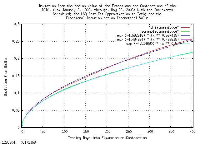
|
Figure X is a plot of the deviation from the median value of the
expansions and contractions of the scrambled Brownian Motion, (random
walk,) equivalent of the DJIA, from January 2, 1900, through, May 26,
2006, and its simulation. 0.010947 * sqrt
(x) is the theoretical value. Note that comparing with
Figure
VI, the deviation is, within numerical precision, very close the
the theoretical value.
The distribution of the marginal increments of the scrambled Brownian Motion, (random walk,) equivalent of the DJIA are the same as shown in Figure III, above, since they are the same increments.
How good is the Laplacian distributed marginal increment approximation?
To get an idea, compare the PDF tail with the empirical tail using the formula for the PDF:
exp (0.710298 - (abs (x) * 147.146009))
The deviation would be:
sqrt (2) / 147.146009 = 0.009610954
There were 29015 trading days
represented in the time series for the DJIA, and 1 /
29015 = 0.000034464, so, the value
0.07466,
(7.7682 deviations, the largest expected
marginal increment in the PDF,) should be represented in the time
series about once, (e.g., exp (0.710298 - (abs (0.07466)
* 147.146009)) = 0.000034464). Any more would be excess
"fat tails," which the model did not handle appropriately. Sorting by
the value of marginal increments:
tsfraction -t "djia" | cut -f1 > "1.temp"
tsfraction -t "djia" | cut -f2 > "2.temp"
paste "2.temp" "1.temp" | sort -n > "djia.increments"
And editing for those marginal increment values greater than
0.07466:
| Value | Date |
|---|---|
-0.235228 |
19141213 |
-0.226105 |
19871019 |
-0.128207 |
19291028 |
-0.117288 |
19291029 |
-0.113283 |
19211219 |
-0.105631 |
19180920 |
-0.099154 |
19291106 |
-0.087304 |
19330526 |
-0.084035 |
19320812 |
-0.082892 |
19070314 |
-0.080394 |
19871026 |
-0.078433 |
19330721 |
-0.077550 |
19371018 |
0.079876 |
19320610 |
0.087032 |
19311008 |
0.090343 |
19330419 |
0.090758 |
19320506 |
0.091858 |
19320213 |
0.093509 |
19311218 |
0.093563 |
19291114 |
0.094708 |
19320211 |
0.095184 |
19320803 |
0.101488 |
19871021 |
0.106771 |
19330531 |
0.113646 |
19320921 |
0.118652 |
19180919 |
0.118839 |
19211217 |
0.123441 |
19291030 |
0.153418 |
19330315 |
Table I is a list of the 29 marginal
increments of the DJIA, (January 2, 1900, to, May 22, 2006,
inclusive,) that were greater than
0.07466,
(7.7682 deviations.) The
29 represent 29 / 29015 =
0.00099948 or about
0.1%, which would be expected about once
every 1000 trading days, or about once
every 4 years of
253 trading days per year.
Finding the marginal increments that were greater than
0.07466 by year:
cut -f2 "djia.increments" | sed 's/[0-9][0-9][0-9][0-9]$//' | \
sort -n | tscount | sort -n
| Number in Year | Year |
|---|---|
1 |
1907 |
1 |
1914 |
1 |
1937 |
2 |
1918 |
2 |
1921 |
2 |
1931 |
3 |
1987 |
5 |
1929 |
5 |
1933 |
7 |
1932 |
Table II is a list of the 29 marginal
increments of the DJIA, (January 2, 1900, to, May 22, 2006,
inclusive,) that were greater than
0.07466,
(7.7682 deviations,) by year in which
the excessive marginal increment occurred. Notice the extreme
clustering in the Great Depression; if it was a random process, we
would expect to see the excessive increments about once every four
years, yet 1932 had seven, and there were seventeen between 1929 and
1933, an order of magnitude and a half too many.
Hand editing for the month in which excessive marginal increments occurred:
| Number in Month | Month |
|---|---|
1 |
04 |
1 |
06 |
1 |
07 |
2 |
02 |
2 |
03 |
2 |
08 |
2 |
11 |
3 |
05 |
3 |
09 |
4 |
12 |
8 |
10 |
Table III is a list of the 29
marginal increments of the DJIA, (January 2, 1900, to, May 22, 2006,
inclusive,) that were greater than
0.07466,
(7.7682 deviations,) by month in which
the excessive marginal increment occurred. Notice the clustering in
October; if it was a random process, we would expect to see the
excessive increments about 29 / 12 =
2.417 times a month, yet October had eight-about a
factor of 3 too many, (the beginning of calendar Q4 is when fund
managers-managing about 60% of equities in the US equity markets-sell
off their losers for the year for tax purposes; so this may be a
structural issue.)
It is doubtful that an analytic function PDF with a finite
variance, (even if stable,) will model the clustered excessive
increments adequately-and addressing the issues will have to be left
to experienced judgment. It is worth noting, however, that the market
does correct itself of excessive increments; the sum of the negative
excessive increments, (13 of them,) in
the DJIA's daily close for 106 years is
-1.515504; the sum of the positive
excessive increments, (16 of them,) is
1.653086, almost totally cancelling, in
the extreme long run. (Or, as a geometric progression, the negative
excessive marginal increments was
0.195027, and the positive
4.811824, for a factor of
0.195027 * 4.811824 = 0.9384, which is
remarkable considering the DJIA increased by a factor of
11125.32 / 68.13 = 163.30 in the
106 years.) It may well be that a
survival strategy for a once-in-four years excessive marginal
increment cluster is appropriate, (but that is not easy; for example,
during the Great Depression, the DJIA was a maximum of 381.17 on
September 3, 1929, and deteriorated to a minimum for the century of
41.22 on July 8, 1932-about 3 years later-and did not recover to its
original maximum until November 23, 1954 when it hit 382.74-about a
quarter of a century later; and that is not adjusted for
inflation.)
The annual market inefficiencies would be difficult to exploit,
(they only happen once a year,) except as a defensive
strategy. However, the short term inefficiencies do offer an
opportunity. Rerunning the script
with an LSQ of only a few days:
R="0.5"
#
> "log"
#
LAST="NOTHING"
#
LOOP="1"
#
while [ "${LOOP}" -eq "1" ]
do
tsmath -l djia | tsderivative | tsmath -s 0.000176 | tsintegrate | \
tsrunmagnitude -r "${R}" > "djia.magnitude"
cut -f1 "djia.magnitude" | tsmath -l > "temp.9"
cut -f2 "djia.magnitude" | tsmath -l > "temp.10"
LAST=`paste temp.9 temp.10 | egrep '^[0]\.' | tslsq -p`
echo "${LAST}"
R=`echo "${LAST}" | sed -e 's/^.* //' -e 's/t.*$//'`
#
if grep -e "${LAST}" "log"
then
LOOP="0"
fi
#
mv "temp.9" "temp.9.last"
mv "temp.10" "temp.10.last"
mv "djia.magnitude" "djia.magnitude.last"
echo "${LAST}" >> "log"
done
The output of the script
fragment is:
-4.510133 + 0.518242t
-4.539663 + 0.521663t
-4.545016 + 0.522309t
-4.546053 + 0.522481t
-4.546241 + 0.522468t
-4.546241 + 0.522468t
-4.546241 + 0.522468t
Meaning that there is a little over a 2% chance that what happened in the DJIA on any given day will happen on the next day, also.
This analysis was originally used to design the algorithm used in
the -d5 option to the tsinvest
program. Checking:
sed 's/^/DJIA /' djia | tsnumber | tsinvest -r | tail -1
# DJIA, p = 0.510810, f = 0.010949, h = 0.544745, i = 68.130000
tsinvestsim djia.sim 29010 | tsinvest -r | tail -1
# DJIA, p = 0.511489, f = 0.010994, h = 0.548321, i = 31.787033
Numbers which agree very favorably with this analysis. And, running the program on the DJIA time series, from January 2, 1900, through, May 26, 2006:
sed 's/^/DJIA /' djia | tsnumber | tsinvest -its -d5 | egrep DJIA | cut -f3 | tsgain -p
1.000535
The theoretical gain, g, per trading
day would be, (from: Equation
(1.20)):
rms = e^(-4.546241) = 0.0106070013
P = 0.522468
g = ((1 + 0.0106070013)^0.522468) * ((1 - 0.0106070013)^(1 - 0.522468))
g = 1.0004204851
The reason the measured daily gain,
g, is larger than the
theoretical value is the sophistication of the algorithm used
in the tsinvest
program-it maintains two different tables, (one probability density
function for positive movements, another for negative,) and calculates
the probabilities of future movements using the empirically derived
probability density functions, (as opposed to the LSQ approximation of
daily returns for a year used in this analysis.) But the theoretical
and empirical values are reasonably close.
Compare these values with the gain of the DJIA, from January 2, 1900, through, May 26, 2006:
tsgain -p djia
1.000176
Which would be the long term investment potential of the DJIA, (from Equation (1.24)):
avg
= 0.000236
rms = 0.010950
P = ((0.000236 / 0.010950) + 1) / 2 = 0.51077626
g = ((1 + 0.010950)^0.51077626) * ((1 - 0.010950)^(1 - 0.51077626))
g = 1.0001760701
The difference in annual gain is significant. Exploiting short term
market inefficiencies resulted in an annual gain, (of 253 trading
days,) of 1.000535^253 =
1.1449017271, or a little less than 15% per
year. Compared with 1.000176^253 =
1.0455301549, or a little less than 5% per year
as a long term investment.
There are other engineered solutions for increasing the value of investments in the DJIA equities, too-as explained in Quantitative Analysis of Non-Linear High Entropy Economic Systems V-specifically, see a simulation of the strategy, which yielded a little over a 17% annual growth in value over the last quarter of the Twentieth Century.
It is interesting to note that, in the long run, a well executed long term portfolio strategy-specfically, rebalancing expeditiously-is more important than timing the market, (which is what this analysis was about,) which, in turn, is more important than picking winners.
A well designed strategy does all three, but in that order of priority.
|
As a side bar, this is the intended usage of the
A word of caution, however. The program is a tool, and a tool is no better than the mechanic using it. It is not a substitute for due diligence and meticulous research. It would probably be better to view the program as a search mechanism for investments-like a Google of the ticker, where one searches for equities/investments that fit a search criteria, (i.e., an investment strategy.) It is a tool for extending the depth and breadth, (and speed,) of investing. |
A note about the DJIA time series:
From 1895, the inception of the DJIA, (although this analysis started with January 2, 1900,) until 1953, trading used 6 day, (actually, five and a half-but even that varied,) weeks-after 1953, 5 day weeks were used; about half of the century's data had 6/5's as many trading days per year in the time series. The number of holidays when the exchanges closed varied over the century, too.
Prior to 2001, equity values were listed in fractions of 1/8'th dollar, (i.e., from the pieces of eight tradition of the NYSE.) After 2001, values were expressed in decimal values, i.e., 1/100'th of a dollar, or a penny.
The DJIA is made up of 30 equities, and the equities are changed to represent the market environment; for example, only GE has a been a constituent part of the DJIA since its inception.
The market inefficiencies have evolved over the century due to the advent of programmed/algorithmic trading. At the beginning of the Twentieth Century, brokers could make handsome profits exploiting the spread, (i.e., arbitrage-since the markets moved at a slower pace,) but at the end of the century, the spread was so small that many brokerage firms had to seek other endeavors-like selling analysis of companies and their equities.
All of these represent anomalies effecting the accuracy of the analysis.
The time series of the DJIA contained 29010 daily closes, (29009
increments.) The margin of error, (using statistical estimation,)
would be 0.010950 / sqrt (29009) =
0.0000642906, meaning that there is a 95% probability,
(i.e., two double sided standard deviations,) that the deviation of
the increments is more than 0.010950 - 0.0000642906 =
0.0108857094, and, less than 0.010950 +
0.0000642906 = 0.011014291, which is about
+/- 0.6%. There is, also, a 95%
probability that the average of the increments is more than
0.000236 - 0.0000642906 = 0.0001717094,
and, less than 0.000236 + 0.0000642906 =
0.0003002906, which is a little more than
+/- 27%, which could be a source of
significant error in the analysis-the average of the increments can
only be known to within a factor of about 2, with a 95% confidence
level. (Note that this uncertainty can be addressed by modifying
P in Equation
(1.24) appropriately to accommodate data set size issues. This is
how the tsinvest
program avoids "chasing bubbles"; its just another
uncertainty that the program has to address).
The distribution of the increments of the Brownian Motion, (random
walk,) equivalent of the DJIA, (see Figure
III,) holds reasonably well through 3 deviations. The Laplacian
distribution used has PDF, (probablity distribution function,) of
e^(x / 0.00679597093) giving a variance
of 2 * 0.00679597093)^2, or a deviation
of 0.00961095426.
The cumulative tail counts would be, (and the actual counts, see Figure IV):
Beyond 3 deviations, there should be 208.46 negative increments and 208.46 positive increments; there were 366 negative increments counted, and 291 positive increments.
Beyond 4 deviations, there should be 50.68 negative increments and 50.68 positive increments; there were 174 negative increments counted, and 130 positive increments.
Beyond 5 deviations, there should be 12.32 negative increments and 12.32 positive increments; there were 88 negative increments counted, and 72 positive increments.
Beyond 6 deviations, there should be 2.99 negative increments and 2.99 positive increments; there were 44 negative increments counted, and 36 positive increments.
Beyond 7 deviations, there should be 0.73 negative increments and 0.73 positive increments; there were 27 negative increments counted, and 20 positive increments.
Note that there is more high order kurtosis than can be explained by the model used. (There are several conjectures: LSQ methodology was used extensively, and with the center of the distribution missing from the data-the most populous data segment-the LSQ approximation could be skewed; there are Levy stable characteristics in the distribution-but the deviation of the increments seems stable, which would be contradictory; there is white noise added to the distribution, possibly created by data collection issues-much of the Twentieth Century collection was done manually-or market overload anomalies created by matching bid/ask failures; yet another conjecture is the assumption, in the model, of a uniform distribution of interday trades.) With so few discrepant data points in the tails, it difficult to make a reliable assessment.
|
As a side bar, note that, for example, the chances of at least
a 5 deviation, (i.e., greater than a 5 sigma hit,) in the
Brownian Motion, (random walk,) equivalent of the DJIA is
0.000000286651571558 using a Gaussian/normal paradigm of the PDF
of the increments, (about 1 in 3,488,556 trading days, or about
once in 13,789 calendar years of 253 trading days per calendar
year-about the duration, so far, of civilization, itself.) The
model used predicts a much greater frequency, about
The Gaussian/normal paradigm is very inappropriate for assessing the risk frequencies of catastrophic events in financial time series-not to mention that high risk daily closes tend to cluster together, (which is what this analysis was about-they are not iid, i.e., statistically independent.) Not to mention that the clusters tend to be synchronous/causal with annual structural phenomena, too. The issue is that any mathematical abstraction should be approached carefully and used with caution-this analysis provides a mathematical model/abstraction of bubbles in financial markets, (look at the graphs, above-that is what they are all about,) which is relatively good. But that does not mean caution is inappropriate. |
To illustrate the ubiquity of time series with geometric progressions, Laplacian distributed increments, and, log-normal evolution, web server page hits will be analyzed-this domain, www.johncon.com, will provide the example. It is not intuitively obvious that server page hits would have these characteristics until it is considered:
For hits to increase over time, the site must be known-and to be known, it has to be bookmarked, (or found by a search engine, or introduced in a mailing list, etc.,) which would lead to more bookmarks, and so on. The probability of a bookmark leading to yet another book mark would remain much the same over time, and if the average probability is greater than unity, the number of hits per day will follow an increasing geometric progression; but there will be significant random variation from day to day, leading to a log-normal evolution over time.
The probability of a hit during any time interval during the day would be approximately constant, leading to Laplacian distributed increments in the time series of web server hits per day.
Finding the median value of page hits per day:
    tslsq -e -p "hits"
    e^(4.948240 + 0.001039t) = 1.001040^(4761.533341 + t) = 2^(7.138801 + 0.001499t
And plotting:
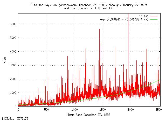
|
Figure XI is a plot of the web server hits per day for domain www.johncon.com, from December 27, 1999, through, January 2, 2007, and its median value, determined by exponential LSQ best fit. (The hits were filtered to exclude crawlers and information robots.)
And, analyzing the increments of the server hits:
    tsmath -l "hits" | tslsq -o | tsderivative | tsnormal -t > "hits.distribution"
    tsmath -l "hits" | tslsq -o | tsderivative | tsnormal -f -t > "hits.frequency"
And plotting:
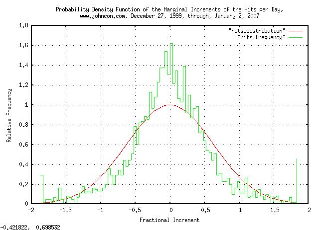
|
Figure XII is a plot of the distribution of the marginal increments of the Brownian Motion, (random walk,) equivalent of the web server hits per day for domain www.johncon.com, from December 27, 1999, through, January 2, 2007, which should be compared with Figure III, above.
Note the implications of the analysis:
The page hits of the web server sites on the Internet will evolve into a log-normal distribution.
The duration of time (i.e., the median time,) that a site is
the most popular, as measured by the number of hits per day, will be
erf (1 / sqrt (t)), or a little over 4
years, (using years as the time scale.)
The ratio of the number of hits per day of the most popular
site to the median of all sites will diverge as e^sqrt
(t) over time.
The growth in the number of page hits per day will grow exponentially, (although the exponential rate will vary, randomly-even decreasing at times.)
Black Scholes Merton methodology can be used to estimate the severity of a downturn in the markets. The methodology assumes the paradigm that equity prices are a random walk fractal, i.e., starting at any specific time, a Gaussian/Normally distributed random number, (with a standard deviation of about 1% = 0.01, of the current price,) is added to the current price of the equity to get the next day's price, and then a second random number is added to get the third day's price, and so on. (Note that the market's value, over time, is a sum of Gaussian/Normally distributed random numbers under this paradigm.)
For details, see: Section I, Section II, Section III, Section IV, Section V,Section VI and Addendum of this series.
Under this paradigm, the equity's price will have a standard
deviation, at some time t in the future,
of 0.01 * sqrt (t). What this means for,
say, t = 100 days is that the equity's
price will be within one standard deviation, (0.01 *
sqrt (100) = 100% = +/- 50%,) 68% of the time. This is
the statistical metric of the magnitude of an equity's price
bubble, (be it gain, or loss, in value.)
Further, under this paradigm, the chances of the duration of an
equity's price being above, (or below,) its value at a specific time
for at least t many days in the future
is erf (1 / sqrt (t)), which is about
1 / sqrt (t) for t
>> 1. What this means is that for, say, for at
least t = 100 days in the future, the
chances of an equity's price being above, (or below,) its starting
price will be 1 / sqrt (100) = 0.1 =
10%. This is a statistical metric of the duration of
an equity's price bubble, (be it gain, or loss, in
value.)
Using the daily closes of the DJIA, (from Yahoo! Finance, ticker ^DJI,) and cutting out the three major declines of the DJIA in the last century, (starting on September 3, 1929; January 14, 2000; October 9, 2007,) and normalizing to the DJIA's value on October 9, 2007, (i.e., all start at 14,164.53,) to compare the declines:
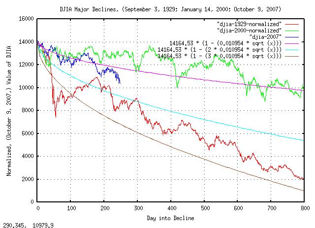
|
Figure XIII is a plot of the DJIA major declines, September 3, 1929; January 14, 2000; October 9, 2007, and, the one, two, and, three standard deviations in the magnitude of the DJIA's contractions, which was found from:
    tsfraction djia | tsavg -p
    0.000230
    tsfraction djia | tsrms -p
    0.010954
Note that the September 3, 1929, decline, (i.e., during the Great Depression,) was about a 2.5 sigma event, (which is about a 1 in 161 chance in any 800 day period.) The January 14, 2000, decline, (i.e., the dot com bubble crash,) was about a 0.625 sigma event, (which has about a 1 in 3.75 chance in any 800 day period.) Extrapolating, it looks like the current financial crisis, (October 8, 2007,) is about a 1.25 sigma event, (which is about a 1 in 9.46 chance in any 800 day period, if it continues.) It would appear, that if the crisis continues, it will be about twice as bad as the January 14, 2000, decline, and about half as bad as the September 3, 1929 decline.
There is a 50% chance, (0.5 = erf (1 / sqrt
(4.4),) that the current crisis, (October 8, 2007,)
will continue at least 4.4 years from October 8, 2007. The chances of
it lasting at least a decade, (32% = 0.32 = 1 / sqrt
(10),) and so on.
So, how bad was the Great Depression?
On September 3, 1929, the DJIA's value was 381.17, the highest until November 23, 1954, when it was 382.74.
On July 8, 1932, the DJIA's value had deteriorated to 41.22, a loss of 89% in value.
During the interval of the decline, (September 3, 1929, to, July 8, 1932,) asset, (including housing,) deflation was about 60%.
During the interval of the decline, the US GDP declined about 40%
In 1932, about 1 in 4 was unemployed
Note that the equity markets, asset values, US GDP, etc., all tend
to track, (but at different rates,) so an assessment can be made,
assuming the current crisis continues, and it will be about half as
bad as the Great Depression. The chances of the current crisis lasting
half as long as the Great Depression, ((1954 - 1929) / 2
= 12.5,) is 1 / sqrt (12.5) = 0.28 =
28% which is about 1 chance in 4, (and a 1 chance in 2
of it lasting 4.4 years.)
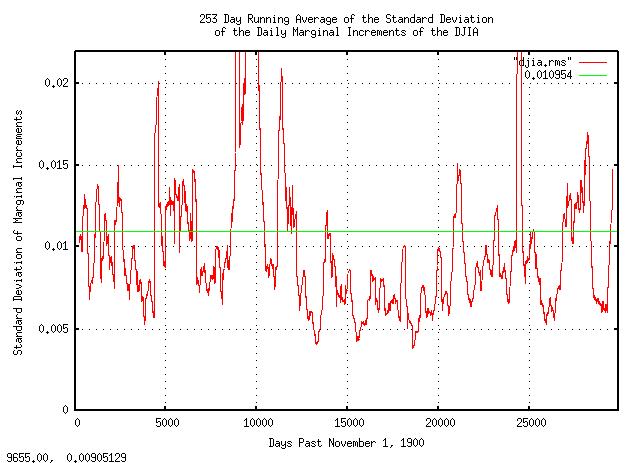
|
Figure XIV is a plot of the 253 day running average of the standard deviation of the daily marginal increments of the DJIA, from November 1, 1900, to October 3, 2008. Note that it was abnormally large in every decline of the DJIA. Observe how the standard deviation of the daily marginal increments effect the following equations:
        avg
        --- + 1
        rms
    P = ------- ........................................(1.24)
           2

                 P          (1 - P)
    g = (1 + rms)  (1 - rms)        ....................(1.20)
Where avg is the arithmetic average
of the marginal increments of an equity market's value,
rms is the standard deviation of the
marginal increments, P is the
probability of an up movement in the marginal increments, (i.e., the
chances a marginal increment will be greater than unity,) and,
g is the average gain of the marginal
increments. (See: Important
Formulas for specifics, and, Section
I of this series for the derivation of the equations.)
Note that rms effects
P, which is the exponent in
g, (avg
varies, too-in the opposite direction of
rms, but it is not as dramatic.) In
point of fact, if rms is double its long
term value, g will be in decline, (i.e.,
be less than unity.) This is the mechanism of market declines, (and
many professional traders use it as a forecasting method for potential
declines and bottoms.) For example, the second largest calendar year
gain in the DJIA was 1933, (69.2697%-right in the middle of the Great
Depression-the largest was 1915, 80.8713%.) Note, also, that the
erf (1 / sqrt (t)) probability of a
bubble's duration means that there is a 50/50 chance of the
duration being longer than 4.4 years, etc., (for example, on July 17,
1990, with a value of 2999.76, the DJIA deteriorated to 2365.10 on
October 11, 1990-in 62 trading days following a three sigma
decline-then recovered in the next 160 trading days, on May 30, 1991.)
So, rms is the mechanism of market
gains, too. (The rms can be too
small-there is an optimal value, in relation to the
avg, see: Section
I.)
In this context, the statement "the current 2008 crisis is a 1.25 sigma event, (i.e., about twice as bad as the 2000 market decline, and, half as bad as the Great Depression, for perspective,) and there is a 50/50 chance that it will be over before 4.4 years from October, 2007, and a 1 in 4 chance that it will last at least 12.5 years," makes reasonable sense.
Note, also, rms is a metric of risk,
and represents the volatility of the equity market, (its also called a
metric of greed by pundits, too.) It is, also, inversely
proportional to confidence in the market, and is the engine
of market bubbles, (in gain, or loss.)
A note about this section. In an effort to keep things simple, traditional Black Scholes Merton methodology was used, which is adequate for short term projections. However, Section III of this series offers a similar, (it uses the same principles,) methodology that is substantially more accurate, in the long term.
The prevailing wisdom is that economic systems are mathematically deterministic and the concepts of classical physics can be used for analysis-such as regression and correlation studies.
A short disproof by contradiction is in order. By building a very
precise simulation of the characteristics of a non-linear dynamical
high entropy economic system with an average of the marginal
increments, avg = 0.0004, and standard
deviation of the marginal increments of rms =
0.02, meaning the system will have an average increase
of 0.04% per day, but it will fluctuate, (with a Gaussian/normal
distribution,) of 2% per day, i.e., the fluctuations will be between
+/- 2% per day, 68% of the time. These numbers are optimal,
(rms^2 = avg,) in the sense that the
growth is maximum, (increasing, or, decreasing, avg, or increasing,
or, decreasing rms, results in lower growth,) and represent the median
values of all equities on all exchanges in the US markets in the 20'th
Century, (about a hundred thousand of them,) most of the developed
countries GDPs, precious metal prices, currency values and exchange
rates, commodity prices, and, asset prices, (like housing,) etc. The
simulation will be provided by the tsinvestsim
program from the NtropiX site.
Calculating P, the probability of an
up movement on any given day:
        avg
        --- + 1
        rms
    P = ------- ........................................(1.24)
           2

    P = 0.51
The control file for the tsinvestsim
program, example.0004.02:
example f = 0.02, p = 0.51
And simulating:
tsinvestsim example.0004.02 90000 | cut -f3 > example.0004.02.ticker
And analyzing:
    tsfraction example.0004.02.ticker | tsavg -p
    0.000402
    tsfraction example.0004.02.ticker | tsrms -p
    0.019936
Which are within a percent of what they should be. And, plotting:
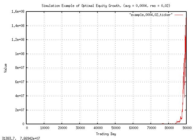
|
Figure XV is a plot of the optimal equity growth simulation. The growth is about a factor of 1.0002 per day, which is about 5% per year, (the simulation is for 90,000 days-about 356 years-to provide a large data set for numerical accuracy.) Note that there are 51 up movements every hundred days, on average, and the average increase per day, 0.0004, is greater than zero; these two number provide the growth in value.
But is it always true?
Changing the metric of risk, rms =
0.03 by 1%, (an increase of 50%,) and calculating
P, the probability of an up movement on
any given day:
        avg
        --- + 1
        rms
    P = ------- ........................................(1.24)
           2

    P = 0.506666666
The control file for the tsinvestsim
program, example.0004.03:
example f = 0.03, p = 0.506666666
And simulating:
tsinvestsim example.0004.03 90000 | cut -f3 > example.0004.03.ticker
And analyzing:
    tsfraction example.0004.02.ticker | tsavg -p
    0.000404
    tsfraction example.0004.02.ticker | tsrms -p
    0.029921
Which are, again, within a percent of what they should be. Note there are still more up movements every hundred days, (50.7-about 3 per 510 less than before, but still more,) on average, and the average increase per day, 0.0004, is what it was before, (and is greater than zero.)
And plotting:
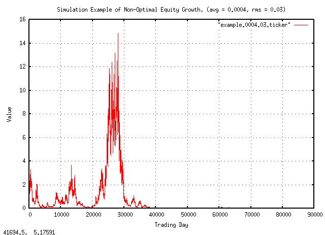
|
Figure XVI is a plot of the non-optimal equity growth simulation. The growth is negative; after building to a value of 15, the equity goes bust about half way through the simulation. Compare with the previous simulation when at 356 years, the equity was worth about $140 million!
It is, indeed, counter intuitive that a stock that moves up more times than it goes down, and has a positive average gain, can deteriorate in value to nothing.
Here is what happened, in detail.
The first simulation, (optimal equity value growth):
                 P          (1 - P)
    g = (1 + rms)  (1 - rms)        ....................(1.20)

                  0.51           (1 - 0.51)
    g = (1 + 0.02)     (1 - 0.02)

            0.51     0.49
    g = 1.02     0.98

    g = 1.0101505 * 1.009750517

    g = 1.0002
Which is positive growth. And, for the second simulation, (non-optimal equity value growth):
                 P          (1 - P)
    g = (1 + rms)  (1 - rms)        ....................(1.20)

                  0.506666666           (1 - 0.506666666)
    g = (1 + 0.03)            (1 - 0.03)

            0.506666666     0.493333334
    g = 1.03            0.97

    g = 1.01508917 * 0.9850858

    g = 0.99995
Which is negative growth.
The intuitive interpretation of the regression analysis was misleading.
Things that fluctuate up more than they fluctuate down, and have a positive average daily gain, do not always increase in value; and the numbers in both simulations are very representative of real world economic phenomena like GDP, equity growth, precious metal values, housing prices, commodity prices, inflation, etc.
The Laplacian Probability Distribution of the marginal increments is ubiquitous in financial time series, (for example, the DJIA, Figure III, above.) The distribution is most pronounced in high speed time series, (day trading, and shorter,) and the deviation of the marginal increments is projected, (via the Central Limit Theorem,) to estimate the Normal/Gaussian probability distribution of the value of an equity, (or other financial instrument,) at some future date-which is quite accurate in the long run.
However, in the short run, the methodology can lead to very optimistic risk assessments.
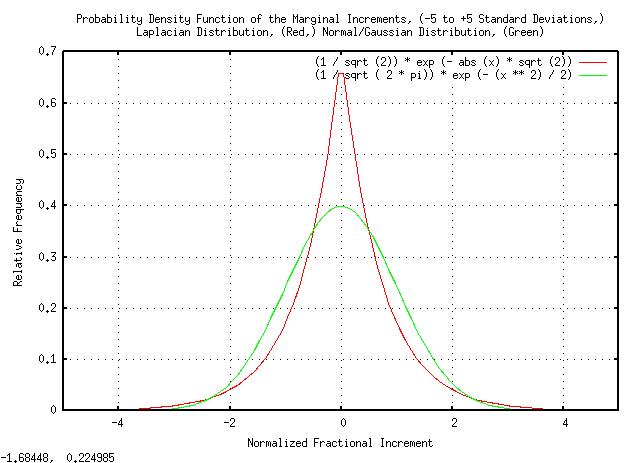
|
Figure XVII is a plot of the Laplacian and the Normal/Gaussian probability distributions, both normalized to unity standard deviation, from -5 standard deviations to +5 standard deviations.
Note there are substantially more small increments in the Laplacian than the Normal/Gaussian distribution below one standard deviation. And, there are more large increments in the Normal/Gaussian than the Laplacian distribution between one and two standard deviations.
Expanding the plot for better visibility above 2 standard deviations:
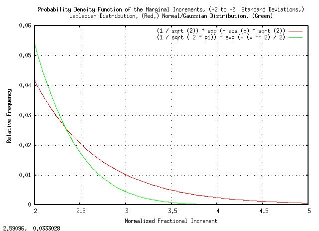
|
Figure XVIII is a plot of the Laplacian and the Normal/Gaussian probability distributions, both normalized to unity standard deviation, from +2 standard deviations to +5 standard deviations.
Note that the frequency of 3 standard deviation increments in the Laplacian is about twice that of the Normal/Gaussian probability distribution-a very substantial error in risk estimation when the value of the risk should be known to better than 1% accuracy.
|
As a side bar, Black Swans do exist in financial time series. What's the frequency of seven standard deviation movements in the daily increments of financial time series using a Normal/Gaussian probability distribution? About once every three billion years. And, the frequency of seven standard deviation movements for the Laplacian probability distribution? More than once a century. Interestingly, the cumulative distribution function of the Laplacian probability distribution is in very reasonable agreement with the number and magnitude of large increment Black Swan movements in the DJIA, Figure III, analyzed, above. The point is that, although the Normal/Gaussian probability distribution/Central Limit Theorem can be a very accurate methodology for estimating the distribution of asset values in the long term, one has to survive the short term Black Swan incremental movements first-and the risks are actually much higher than predicted by the Normal/Gaussian distributed short term increments assumption. |
--

John Conover, john@email.johncon.com, http://www.johncon.com/